
Possibilities of Real Time Monitoring of Micropollutants in Wastewater Using Laser-Induced Raman & Fluorescence Spectroscopy (LIRFS) and Artificial Intelligence (AI)

 , , and
Abstract
:1. Introduction
2. Fundamentals
2.1. Fluorescence/Raman Spectroscopy
2.2. Wastewater Treatment and Monitoring

3. Equipment
3.1. Raman/Fluorescence Detection System
4. Data Processing
4.1. Data Preparation

4.2. Substance Classification
5. Methodology and Targets
6. Results
7. Discussion and Conclusions
Author Contributions
Funding
Institutional Review Board Statement
Informed Consent Statement
Data Availability Statement
Acknowledgments
Conflicts of Interest
References
- Sacher, F.; Kümmel VThoma, A.; Fuchs, S.; Kaiser, M.; Lambert, B.; Ullrich, A. Analytik von prioritären Stoffen in Abwasserproben—Eine wichtige Voraussetzung für eine Bestandsaufnahme in deutschen Kläranlagen. Mitt. Umweltchem. Ökotoxikol. 2018, 3, 56–58. [Google Scholar]
- Luo, Y.; Guo, W.; Ngo, H.H.; Nghiem, L.D.; Ibney Hai, F.; Zhang, J.; Liang, S.; Wang, X.C. A review on the occurrence of micropollutants in the aquatic environment and their fate and removal during wastewater treatment. Sci. Total Environ. 2014, 473–474, 619–641. [Google Scholar] [CrossRef] [PubMed]
- Umweltbundesamt. Recommendations for reducing micropollutants in waters. In German Environment Agency Section II; 2.1 General Aspects of Water and Soil; Umweltbundesamt: Dessau, Germany, 2018. [Google Scholar]
- Rasheed, T.; Bilal, M.; Nabeel, F.; Adeel, M.; Iqbal, H.M. Environmentally-related contaminants of high concern: Potential sources and analytical modalities for detection, quantification, and treatment. Environ. Int. 2019, 122, 52–66. [Google Scholar] [CrossRef] [PubMed]
- Loos, R.; Negrão De Carvalho, R.; Comero, S.; Conduto, A.D.; Lettieri, G.M.T.; Locoro, G.; Paracchini, B.; Tavazzi, S.; Gawlik, B.; Blaha, L.; et al. EU Wide Monitoring Survey on Waste Water Treatment Plant Effluents; EUR 25563 EN, JRC76400; Publications Office of the European Union: Luxembourg, 2012; ISBN 978-92-79-26784-0. [Google Scholar]
- WFD Directive 2000/60/EC of the European Parliament and of the Council of 23 October 2000 Establishing a Framework for Community Action in the Field of Water Policy. Available online: https://eur-lex.europa.eu/resource.html?uri=cellar:5c835afb-2ec6-4577-bdf8-756d3d694eeb.0004.02/DOC_1&format=PDF (accessed on 22 April 2022).
- Directive 2008/105/EC Environmental Quality Standards (EQS) Applicable to Surface Water. Available online: https://www.legislation.gov.uk/eudr/2008/105/contents (accessed on 22 April 2022).
- LANUV NRW Untersuchungen zum Eintrag und zur Elimination Gefährlicher Stoffe in Kläranlagen. 2006, Teil 2. Available online: https://scholar.google.com/scholar?hl=en&as_sdt=0%2C5&q=LANUV+NRW+Investigations+on+the+input+and+elimination+of+hazardous+substances+in+sewage+treatment+plants&btnG= (accessed on 14 June 2022).
- Umweltbundesamt. Maßnahmen zur Verminderung des Eintrages von Mikroschadstoffen in die Gewässer—Phase 2. Texte 60. Available online: https://www.umweltbundesamt.de/sites/default/files/medien/377/publikationen/mikroschadstoffen_in_die_gewasser-phase_2.pdf2016 (accessed on 14 June 2022).
- Geissen, V.; Mol, H.; Klumpp, E.; Umlauf, G.; Nadal, M.; Van Der Ploeg, M.; van de Zee, S.E.A.T.M.; Ritsema, C.J. Emerging pollutants in the environment: A challenge for water resource management. Int. Soil Water Conserv. Res. 2015, 3, 57–65. [Google Scholar] [CrossRef]
- Wanda, E.; Nyoni, H.; Mamba, B.; Msagati, T. Occurrence of emerging micropollutants in water systems in Gauteng, Mpumalanga, and North West Provinces, South Africa. Int. J. Environ. Res. Public. Health 2017, 14, 79. [Google Scholar] [CrossRef] [PubMed] [Green Version]
- Ahmed, M.B.; Johir, M.A.H.; Ngo, H.H.; Guo, W.; Zhou, J.L.; Belhaj, D.; Moni, M.A. Chapter 4—Methods for the analysis of micro-pollutants. In Current Developments in Biotechnology and Bioengineering; Varjani, S., Pandey, A., Tyagi, R.D., Ngo, H.H., Larroche, C., Eds.; Elsevier: Amsterdam, The Netherlands, 2020; ISBN 9780128195949. [Google Scholar] [CrossRef]
- Schwarzenbach, R.P.; Escher, B.I.; Fenner, K.; Hofstetter, T.B.; Johnson, C.A.; von Gunten, U.; Wehrli, B. The challenge of micropollutants in aquatic systems. Science 2006, 313, 1072–1077. [Google Scholar] [CrossRef] [PubMed]
- Kumar, N.M.; Sudha, M.C.; Damodharam, T.; Varjani, S. Micro-pollutants in surface water: Impacts on the aquatic environment and treatment technologies. In Current Developments in Biotechnology and Bioengineering; Emerging Organic Micro-pollutants; Elsevier: Amsterdam, The Netherlands, 2020; Chapter 3; pp. 41–62. [Google Scholar] [CrossRef]
- Wichern, M.; Heinz, E. Abwassertechnisches Laborpraktikum “Forschungspraktikum Siedlungswasserwirtschaft”. Lehrstuhl für Siedlungswasserwirtschaft und Umwelttechnik, Ruhr Universität Bochum. Abwassertechnisches Laborpraktikum Forschungspraktikum Siedlungswasserwirtschaft—PDF Free Download. 2017. Available online: docplayer.org (accessed on 14 June 2022).
- Alvarino, T.; Suarez, S.; Lema, J.; Omil, F. Understanding the sorption and biotransformation of organic micropollutants in innovative biological wastewater treatment technologies. Sci. Total Environ. 2017, 615, 297–306. [Google Scholar] [CrossRef]
- Chavoshani, A.; Hashemi, A.; Amin, M.M.; Ameta, S.C. Micropollutants and Challenges: Emerging in the Aquatic Environments and Treatment Processes; Elsevier: Amsterdam, The Netherlands, 2020; Chapter 1; ISBN 978-0-12-818612-1. [Google Scholar] [CrossRef]
- Tijani, J.; Fatoba, O.; Petrik, L.F. A Review of pharmaceuticals and endocrine-disrupting compounds: Sources, effects, removal, and detections. Water Air Soil Pollut. 2013, 224, 1170. [Google Scholar] [CrossRef] [Green Version]
- IKSR. Auswertungsbericht Biozide und Korrosionsschutzmittel. Nr. 183; Internationale Kommission zum Schutze des Rheins: Koblenz, Germany, 2010; ISBN 3-941994-15-8. [Google Scholar]
- Abegglen, C.; Escher, B.; Hollender, J.; Koepke, S.; Ort, C.; Peter, A.; Siegrist, H.; von Gunten, U.; Zimmermann, S.G.; Koch, M.; et al. Ozonung von Gereinigtem Abwasser. Schlussbericht Pilotversuch Regensdorf. Studie der Eawag im Auftrag des BAFU und des AWEL. Eidgenössische Anstalt für Wasserversorgung, Abwasserreinigung und Gewässerschutz. Zürich. 2009. Available online: http://spurenstoffelimination.de/files/Ozonung_Abwasser_Schlussbericht_Regensdorf.pdf (accessed on 4 April 2022).
- Miehe, U. Wirksamkeit technischer Barrieren zur Entfernung von anthropogenen Spurenstoffen—Kläranlagen und Raumfilt. Ph.D. Dissertation, Technischen Universität Berlin, Berlin, Germany, 2016. [Google Scholar]
- Böhler, M.; Siegrist, H. Aktivkohledosierung in den Zulauf zur Flockungs-Sandfiltration Kläranlage Kloten/Opfikon—Grosstechnische Umsetzung im Rahmen ergänzender Untersuchungen zum MicroPoll-Projekt. DWA-Seminar Weitergehende Abwasserreinigung. Bonn, 18.01.2011. In Maßnahmen zur Verminderung des Eintrages von Mikroschadstoffen in die Gewässer—Phase 2; Texte 60/2016; UBA: Dessau-Roßlau, Germany, 2016. [Google Scholar]
- Grünebaum, T. Elimination von Arzneimittelrückständen in kommunalen Kläranlagen. Elimination von Arzneimitteln und organischen Spurenstoffen: Entwicklung von Konzeptionen und innovativen, kostengünstigen Reinigungsverfahren. Schlussbericht Phase 1. Düsseldorf: Ministerium für Klimaschutz, Umwelt, Landwirtschaft, Natur- und Verbraucherschutz des Landes Nordrhein-Westfalen. In Maßnahmen zur Verminderung des Eintrages von Mikroschadstoffen in die Gewässer—Phase 2; Texte 60/2016; UBA: Dessau-Roßlau, Germany, 2016. [Google Scholar]
- Bornemann, C.; Erbe, V.; Hachenberg, M.; Kolisch, G.; Osthoff, T.; Taudien, Y. Einsatz von Pulveraktivkohle in vorhandene Flockungsfiltrationsanlagen am Beispiel der Kläranlage Buchenhofen. Tagungsband, Gesellschaft zur Förderung der Siedlungswasserwirtschaft an der RWTH Aachen (45. Essener Tagung für Wasser- und Abfallwirtschaft). In Maßnahmen zur Verminderung des Eintrages von Mikroschadstoffen in die Gewässer—Phase 2; Texte 60/2016; UBA: Dessau-Roßlau, Germany, 2016. [Google Scholar]
- Crane, M.; Watts, C.; Boucard, T. Chronic aquatic environmental risks from exposure to human pharmaceuticals. Sci. Total Environ. 2006, 367, 23–41. [Google Scholar] [CrossRef]
- Malaj, E.; von der Ohe, P.C.; Grote, M.; Kühne, R.; Mondy, C.P.; Usseglio-Polatera, P.; Brack, W.; Schäfer, R.B. Organic chemicals jeopardize the health of freshwater ecosystems on the continental scale. Proc. Natl. Acad. Sci. USA 2014, 111, 9549–9554. [Google Scholar] [CrossRef] [Green Version]
- Prasse, C.; Stalter, D.; Schulte-Oehlmann, U.; Oehlmann, J.; Ternes, T.A. Spoilt for choice: A critical review on the chemical and biological assessment of current wastewater treatment technologies. Water Res. 2015, 87, 237–270. [Google Scholar] [CrossRef] [PubMed] [Green Version]
- Diehle, M.; Gebhardt, W.; Pinnekamp, J.; Schäffer, A.; Linnemann, V. Ozonation of valsartan: Structural elucidation and environmental properties of transformation products. Chemosphere 2019, 216, 437–448. [Google Scholar] [CrossRef] [PubMed]
- Jiang, J.; Zhou, Z.; Sharma, V.K. Occurrence, transportation, monitoring and treatment of emerging micro-pollutants in waste water — A review from global views. Microchem. J. 2013, 110, 292–300. [Google Scholar] [CrossRef]
- O’Flynn, D.; Lawler, J.; Yusuf, A.; Parle-McDermott, A.; Harold, D.; Mc Cloughlin, T.; Holland, L.; Regan, F.; White, B. A review of pharmaceutical occurrence and pathways in the aquatic environment in the context of a changing climate and the COVID-19 pandemic. Anal. Methods 2021, 13, 575. [Google Scholar] [CrossRef]
- Daughton, C.G.; Ternes, T.A. Pharmaceuticals and personal care products in the environment: Agents of subtle change? Environ. Health Perspect. 1999, 107 (Suppl. S6), 907–938. [Google Scholar] [CrossRef] [PubMed]
- Jjemba, P.K. Excretion and ecotoxicity of pharmaceutical and personal care products in the environment. Ecotoxicol. Environ. Saf. 2006, 63, 113–130. [Google Scholar] [CrossRef]
- Petrie, B.; Barden, R.; Kasprzyk-Hordern, B. A review on emerging contaminants in wastewaters and the environment: Current knowledge, understudied areas and recommendations for future monitoring. Water Res. 2015, 72, 3–25. [Google Scholar] [CrossRef]
- Schmidt, T.C. Recent trends in water analysis triggering future monitoring of organic micropollutants. Anal. Bioanal. Chem. 2018, 410, 3933–3941. [Google Scholar] [CrossRef] [Green Version]
- Helmenstine, A.-M. Spectroscopy Introduction. Thought Co. 26 August 2020. Available online: https://www.thoughtco.com/introduction-to-spectroscopy-603741 (accessed on 22 April 2022).
- Sapkota, Anupama. 22 Types of Spectroscopy with Definition, Principle, Steps, Uses. 12 January 2022. Available online: https://microbenotes.com/types-of-spectroscopy/ (accessed on 23 April 2022).
- Kierat, R.M. Synthese, Modifikation und Biologische Anwendung Fluoreszierender Xanthenfarbstoffe. Inaugural Dissertation, Ruprechts-Karls-Universität Heidelberg, Heidelberg, Germany, 2008. Available online: http://www.ub.uni-heidelberg.de/archiv/8301 (accessed on 28 January 2022).
- Sauer, M.; Hofkens, J.; Enderlein, J. Handbook of Fluorescence Spectroscopy and Imaging: From Single Molecules to Ensembles; Wiley: Hoboken, NJ, USA, 2011. [Google Scholar] [CrossRef]
- Lakowicz, J.R. Principles of Fluorescence Spectroscopy; Springer: London, UK, 2010. [Google Scholar] [CrossRef]
- Chinen, A.; Guan, C.; Ferrer, J.; Barnaby, S.; Merkel, T.; Mirkin, C. Nanoparticle Probes for the Detection of Cancer Biomarkers, Cells, and Tissues by Fluorescence. Chem. Rev. 2015, 115, 10530–10574. [Google Scholar] [CrossRef] [Green Version]
- Schrader, B. Chemische Anwendungen der Raman-Spektroskopie. Angew. Chem. 1973, 85, 925–950. [Google Scholar] [CrossRef]
- Vandenabeele, P. Practical Raman spectroscopy: An introduction. In The Atrium Southern Gate Chichester West Sussex United Kingdom; Wiley: Hoboken, NJ, USA, 2013. [Google Scholar]
- Post, C.; Brülisauer, S.; Waldschläger, K.; Hug, W.; Grüneis, L.; Heyden, N.; Schmor, S.; Förderer, A.; Reid, R.; Reid, M.; et al. Application of Laser-Induced, Deep UV Raman Spectroscopy and Artificial Intelligence in Real-Time Environmental Monitoring—Solutions and First Results. Sensors 2021, 21, 3911. [Google Scholar] [CrossRef] [PubMed]
- Asher, S.A.; Johnson, C.R. A new selective technique for characterization of polycyclic aromatic hydrocarbons in complex samples: UV resonance Raman spectroscopy of coal liquids. Anal. Chem. 1984, 56, 2258–2261. [Google Scholar]
- Liu, C. Implementation of Deep Ultraviolet Raman Spectroscopy. Ph.D. Thesis, Technical University of Denmark, Kongens Lyngby, Denmark, 2011. [Google Scholar]
- Photon Systems Inc. (Ed.) DUV Raman PL200. Fully Integrated, Lab Model Deep UV Resonance Raman & Photoluminescence Spectrometer, with Microscopic Imaging. 2017. Available online: https://photonsystems.com/wp-content/uploads/2019/02/DUV-RamanPL200-Data-Sheet-V12-Web.pdf (accessed on 10 February 2022).
- Photon Systems Inc. (Ed.) New Deep UV Raman & Photoluminescence Spectrometer System: The DUV Raman/PL 200. In Proceedings of the SPIE DCS 2018, Orlando, FL, USA, 17–19 April 2018. [Google Scholar]
- Photon Systems Inc. (Ed.) Fused Fluorescence and Raman—Photon Systems, 9.3.2020. 2017. Available online: https://photonsystems.com/fused-fluorescence-and-Raman/ (accessed on 10 February 2022).
- Henderson, R.K.; Baker, A.; Murphy, K.R.; Hambly, A.; Stuetz, R.M.; Khan, S.J. Fluorescence as a potential monitoring tool for recycled water systems: A review. Water Res. 2009, 43, 863–881. [Google Scholar] [CrossRef]
- Spencer, R.G.M.; Bolton, L.; Baker, A. Freeze/thaw and pH effects on freshwater dissolved organic matter fluorescence and absorbance properties from a number of UK locations. Water Res. 2007, 42, 2941–2950. [Google Scholar] [CrossRef] [PubMed]
- Baker, A.; Cumberland, S.A.; Bradley, C.; Buckley, C.; Bridgeman, J. To what extent can portable fluorescence spectroscopy be used in the real-time assessment of microbial water quality? Sci. Total Environ. 2015, 532, 14–19. [Google Scholar] [CrossRef] [PubMed] [Green Version]
- Reynolds, D.M.; Ahmad, S.R. The effect of metal ions on the fluorescence of sewage wastewater. Water Res. 1995, 29, 2214–2216. [Google Scholar] [CrossRef]
- BMUV Kurzinfo Abwasser—Kläranlage. Available online: https://www.bmuv.de/en/topics/water-resources-waste/water-management/wastewater/sewage-treatment-plant (accessed on 4 April 2022).
- Sonnenburg, A.; Mosbach, J.; Grimmel, O.; Urban, W. Leistungssteigerung von Sandfängen. Wien. Mitt. 2020, 252, 91–112. Available online: https://repositum.tuwien.at/bitstream/20.500.12708/15607/1/sonnenburg_leistungssteigerung%20von%20sandf%c3%a4ngen.pdf (accessed on 3 February 2022).
- Engelhardt, M.; Wagner, M.; Behnisch, J.; Blach, T.; Schwarz, M. Abwassertechnik. In Handbuch für Bauingenieure; Zilch, K., Diederichs, C.J., Beckmann, K.J., Gertz, C., Malkwitz, A., Moormann, C., Eds.; Springer Fachmedien: Wiesbaden, Germany, 2020. [Google Scholar]
- Gupta, V.K.; Ali, I.; Saleh, T.A.; Nayaka, A.; Agarwal, S. Chemical treatment technologies for waste-water recycling—An overview. RSC Adv. 2012, 2, 6380–6388. [Google Scholar] [CrossRef]
- Franklin, L.B. Wastewater Engineering: Treatment. Disposal and Reuse; McGraw Hill, Inc.: New York, NY, USA, 1991. [Google Scholar]
- Rosenwinkel, K.; Kroiss, H.; Dichtl, N.; Seyfried, C.; Weiland, P. Anaerobtechnik; Springer: Berlin/Heidelberg, Germany, 2015. [Google Scholar]
- Melin, T.; Jefferson, B.; Bixio, D.; Thoeye, C.; De Wilde, W.; De Koning, J.; van der Graaf, J.; Wintgens, T. Membrane bioreactor technology for wastewater treatment and reuse. Desalination 2006, 187, 271–282. [Google Scholar] [CrossRef]
- Förstner, U.; Köster, S. (Eds.) Umweltschutztechnik; Springer: Berlin/Heidelberg, Germany, 2018. [Google Scholar]
- Wolf, Y.; Oster, S.; Shuliakevich, A.; Brückner, I.; Dolny, R.; Linnemann, V.; Pinnekamp, J.; Hollert, H.; Schiwy, S. Improvement of wastewater and water quality via a full-scale ozonation plant?—A comprehensive analysis of the endocrine potential using effect-based methods. Sci. Total Environ. 2022, 803, 149756. [Google Scholar] [CrossRef]
- Radjenović, J.; Petrović, M.; Barceló, D. Advanced mass spectrometric methods applied to the study of fate and removal of pharmaceuticals in wastewater treatment. Trends Anal. Chem. 2007, 26, 1132–1144. [Google Scholar] [CrossRef]
- Fondermann, P. Investigation of Correlation of Selected Amino Acids to Sum Parameters in Monitoring of Wastewater Treatment Plants Using Fluorescence Laser Spectrometry. Master’s Thesis, Department of Engineering Geology and Hydrogeology, RWTH Aachen University, Aachen, Germany, 11 May 2021. [Google Scholar]
- Pinnekamp, J. Grundlagen der Gewässergütewirtschaft und Siedlungswasserwirtschaft. Vorlesungsskript. RWTH Aachen, Lehrstuhl für Siedlungswasserwirtschaft und Wassergütewirtschaft (ISA). 2019. Available online: https://moodle.rwth-aachen.de/pluginfile.php/377447/mod_resource/content/0/GGSW_SS19_V02%20Charakterisierung%20Wasser%20Abwasser_190409 (accessed on 11 April 2021). not publicly accessible.
- Penn, M.R.; Pauer, J.J.; Mihelcic, J.R. Biochemical Oxygen Demand. Encyclopedia of Live Support Systems (EOLSS). 2009. Available online: http://www.eolss.net/sample-chapters/c06/e6-13-04-03.pdf (accessed on 9 April 2021).
- ISO 15705:2002; Water Quality—Determination of the Chemical Oxygen Demand Index (ST-COD)—Small-Scale Sealed-Tube Method. ISO: Geneva, Switzerland, 2002.
- ISO 6060:1989; Water Quality—Determination of the Chemical Oxygen Demand. ISO: Geneva, Switzerland, 1989.
- ISO 3199; Ausgabe 1975-02 Natriumchlorat für Industriezwecke; Bestimmung des Chloratgehaltes; Titrimetrische Dichromat-Methode. ISO: Geneva, Switzerland, 1975.
- Reineke, W.; Schlömann, M. Umweltmikrobiologie, 3rd ed.; Springer Spektrum: Berlin, Germany, 2020. [Google Scholar]
- DIN EN 1484; Water Analysis—Guidelines for the Determination of Total Organic Carbon (TOC) and Dissolved Organic Carbon (DOC). Beuth Verlag: Berlin, Germany, 2019.
- DIN EN 15216:2021-12; Environmental Solid Matrices—Determination of Total Dissolved Solids (TDS) in Water and Eluates. Beuth Verlag: Berlin, Germany, 2021.
- Köppel, S.; Denner, M. DOC/TOC im Eluat von Abfällen aus der MBA. Evaluierung der Bestimmungsverfahren. Wien: Umweltbundesamt GmbH (Report/Umweltbundesamt, [N.F.], p 298). 2010. Available online: https://www.umweltbundesamt.at/fileadmin/site/publikationen/REP0298.pdf (accessed on 29 November 2021).
- Pine, C.S.F. Process gas chromatography. Talanta 1967, 14, 269–297. [Google Scholar] [CrossRef]
- Villalobos, R. Process gas chromatography. Anal. Chem. 1975, 47, 983A–1004A. [Google Scholar] [CrossRef]
- Clemons, J. Chromatography in process analysis. In Encyclopedia of Analytical Chemistry; Wiley: Hoboken, NJ, USA, 2016; pp. 1–27. [Google Scholar] [CrossRef]
- Kessler, R.W. Prozessanalytik; Wiley: Weinheim, Germany, 2006. [Google Scholar]
- Straub, A. Einfache Messmethoden zur Charakterisierung sowie Maßnahmen zur Erhöhung der Zuverlässigkeit und Leistungsfähigkeit biologischer Kleinkläranlagen. Ph.D. Dissertation, Lehrstuhl Wassertechnik und Siedlungswasserbau der Brandenburgischen Technischen Universität Cottbus, Cottbus, Germany, 2008. [Google Scholar]
- EPA. Method 180.1:1993—Determination of Turbidity by Nephelometry; EPA: Washington, DC, USA, 1993. [Google Scholar]
- ISO 7027-1:2016(en); Water Quality—Determination of Turbidity—Part 1: Quantitative Methods. ISO: Geneva, Switzerland, 2016. Available online: https://www.iso.org/standard/62801.html (accessed on 14 June 2022).
- Shi, Z.; Chow, C.W.K.; Fabris, R.; Liu, J.; Jin, B. Applications of Online UV-Vis Spectrophotometer for Drinking Water Quality Monitoring and Process Control: A Review. Sensors 2022, 22, 2987. [Google Scholar] [CrossRef]
- Wortberg, M.; Kurz, J. Analytics 4.0: Online wastewater monitoring by GC and HPLC. Anal. Bioanal. Chem. 2019, 411, 6783–6790. [Google Scholar] [CrossRef]
- Photon Systems Inc. (Ed.) Manual: Raman PL 200; Photon Systems: Covina, CA, USA, 2020; unpublished. [Google Scholar]
- Parthier, R. Messtechnik—Vom SI-Einheitensystem über Bewertung von Messergebnissen zu Anwendungen der Elektrischen Messtechnik, 9th ed.; Springer: Berlin/Heidelberg, Germany, 2020; ISBN 978-3-658-27130-5. [Google Scholar]
- KnowItAll-Software, Spektroskopie-Edition. Available online: https://sciencesolutions.wiley.com/knowitall-software-spektroskopie-edition/?lang=de (accessed on 5 April 2022).
- Görgens, M. Method Comparison of Laser Induced Fluorescence and Raman Spectroscopy Using Water Management Relevant Micropollutants. Master’s Thesis, Department of Engineering Geology and Hydrogeology, RWTH Aachen University, Aachen, Germany, 6 May 2021. [Google Scholar]
- Wongburi, P.; Park, J.K. Big Data Analytics from a Wastewater Treatment Plant. Sustainability 2021, 13, 12383. [Google Scholar] [CrossRef]
- Liu, J.; Osadchy, M.; Ashton, L.; Foster, M.; Solomone, C.; Gibson, S. Deep convolutional networks for Raman spectrum recognition: A unified solution. Analyst 2017, 142, 4067–4074. [Google Scholar] [CrossRef] [Green Version]
- Directive (EU) 2020/2184 of the European Parliament and of the Council of 16 December 2020 on the Quality of Water Intended for Human Consumption. Available online: https://eur-lex.europa.eu/legal-content/EN/TXT/PDF/?uri=CELEX:32020L2184&from=ES (accessed on 22 April 2022).
- Bhartia, R.; Hug, W.; Reid, R. Improved sensing using simultaneous deep UV Raman and fluorescence detection. In Chemical, Biological, Radiological, Nuclear, and Explosives (CBRNE) Sensing XIII (83581A); International Society for Optics Photonics: Bellingham, WA, USA, 2012; Volume 8358. [Google Scholar]
- Reinartz, A. Investigation of Selected Disinfection Byproducts (DNP) in Ozonation of Wastewater Treatment Plants by Laser-Induced Raman and Fluorescence Spectroscopy—Possibilities and Limitations of Application. Master’s Thesis, Department of Engineering Geology and Hydrogeology, RWTH Aachen University, Aachen, Germany, 31 March 2022. [Google Scholar]
- Ahmad, S.R.; Reynolds, D.M. Synchronous fluorescence spectroscopy of wastewater and some potential constituents. Water Res. 1995, 20, 1599–1602. [Google Scholar] [CrossRef]
- Bridgeman, J.; Baker, A.; Carliell-Marquet, C.; Carstea, E.M. Determination of changes in wastewater quality through a treatment works using fluorescence spectroscopy. Environ. Technol. 2013, 34, 3069–3077. [Google Scholar] [CrossRef]
- Carstea, E.M.; Popa, C.L.; Baker, A.; Bridgeman, J. In situ fluorescence measurements of dissolved organic matter: A review. Sci. Total Environ. 2020, 699, 134361. [Google Scholar] [CrossRef]
- Sharpe, T.J. Assessing a Fluorescence Spectroscopy Method for In-Situ Microbial Drinking Water Quality. Ph.D. Dissertation, Portland State University, Portland, OR, USA, 2017. [Google Scholar] [CrossRef] [Green Version]
- Cumberland, S.; Bridgeman, J.; Baker, A.; Sterling, M.; Ward, D. Fluorescence spectroscopy as a tool for determining microbial quality in potable water applications. Environ. Technol. 2012, 33, 687–693. [Google Scholar] [CrossRef]
- Mohrdieck, M. Optimierung von Wasseraufbereitungsprozessen über ein Echtzeit-Monitoring von Summenparametern mit Hilfe der Fluoreszenz-Laserspektroskopie. Master’s Thesis, Department of Engineering Geology and Hydrogeology, RWTH Aachen University, Aachen, Germany, 31 March 2021. [Google Scholar]
- Baldwin, D.S.; Valo, W. Exploring the relationship between the optical properties of water and the quality and quantity of dissolved organic carbon in aquatic ecosystems: Strong correlations do not always mean strong predictive power. Environ. Sci. Process. Impacts 2015, 17, 619–630. [Google Scholar] [CrossRef]
- Kowalczuk, P.; Cooper, W.J.; Durako, M.J.; Kahn, A.E.; Gonsior, M.; Young, H. Characterization of dissolved organic matter fluorescence in the South Atlantic Bight with use of PARAFAC model: Relationships between fluorescence and its components, absorption coefficients and organic carbon concentrations. Mar. Chem. 2010, 118, 22–36. [Google Scholar] [CrossRef]
- Shutova, Y.; Baker, A.; Bridgeman, J.; Henderson, R.K. Spectroscopic characterization of dissolved organic matter changes in drinking water treatment: From PARAFAC analysis to online monitoring wavelengths. Water Res. 2014, 54, 159. [Google Scholar] [CrossRef]
- Schmor, S. Development of Raman Measurement Standards for Selected Substances in Sewage—Conception and Execution of a Flow Experiment. Master’s Thesis, Department of Engineering Geology and Hydrogeology, RWTH Aachen University, Aachen, Germany, 30 April 2020. [Google Scholar]
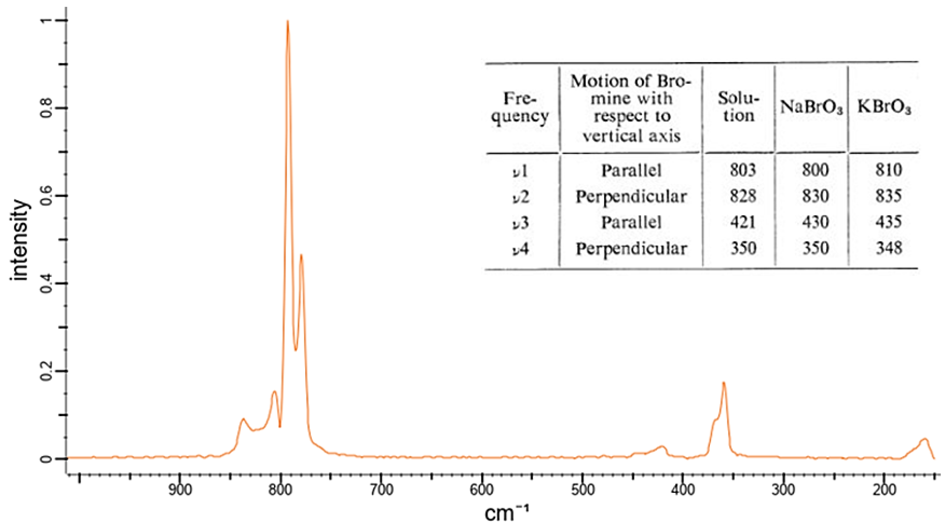
- Radhakrishna, S.; Karguppikar, A.M. Raman Spectra of Irradiated Alkali Bromate Crystals. J. Phys. Soc. Jpn. 1973, 2, 578–581. [Google Scholar] [CrossRef]


| Substance; CAS no. | Manufacturer | Measurement | Concentration | Legal Limits |
|---|---|---|---|---|
| Metformin hydrochloride; 1115-70-4; purity > 99% | BioTrend, Cologne, Germany | Pure powder in solution with cuvette from Starna Cells® Atascadero, CA, USA | Pure substance and 10; 1; 0.1; 0.01 g/L in solution with Millipore®, Merck KGaA Darmstadt, Germany | Preventive value 0.1 µg/L ° |
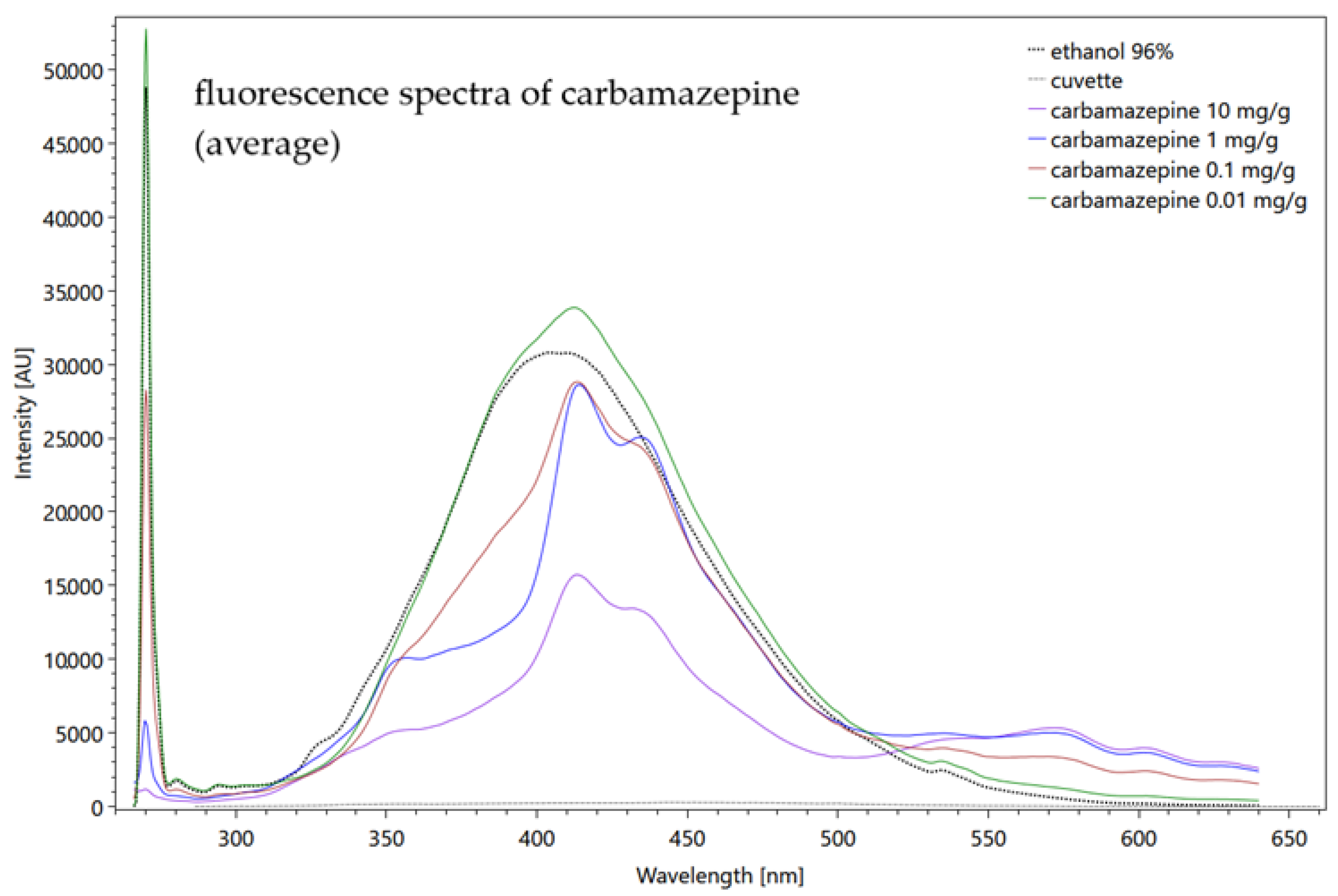
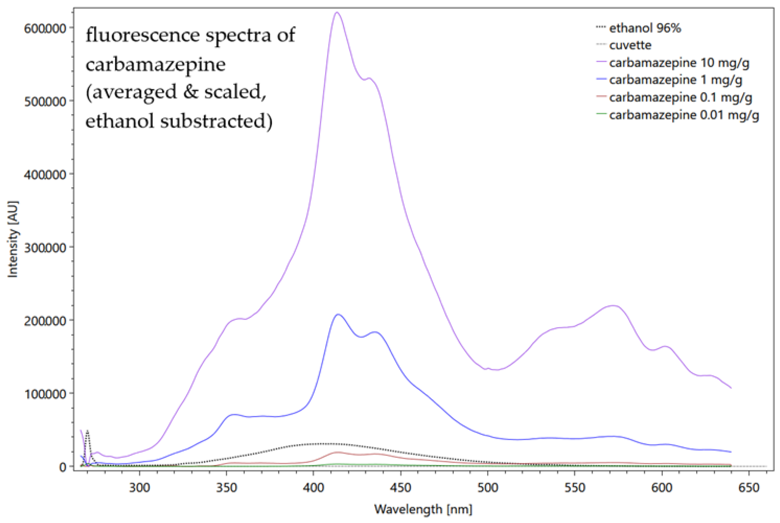
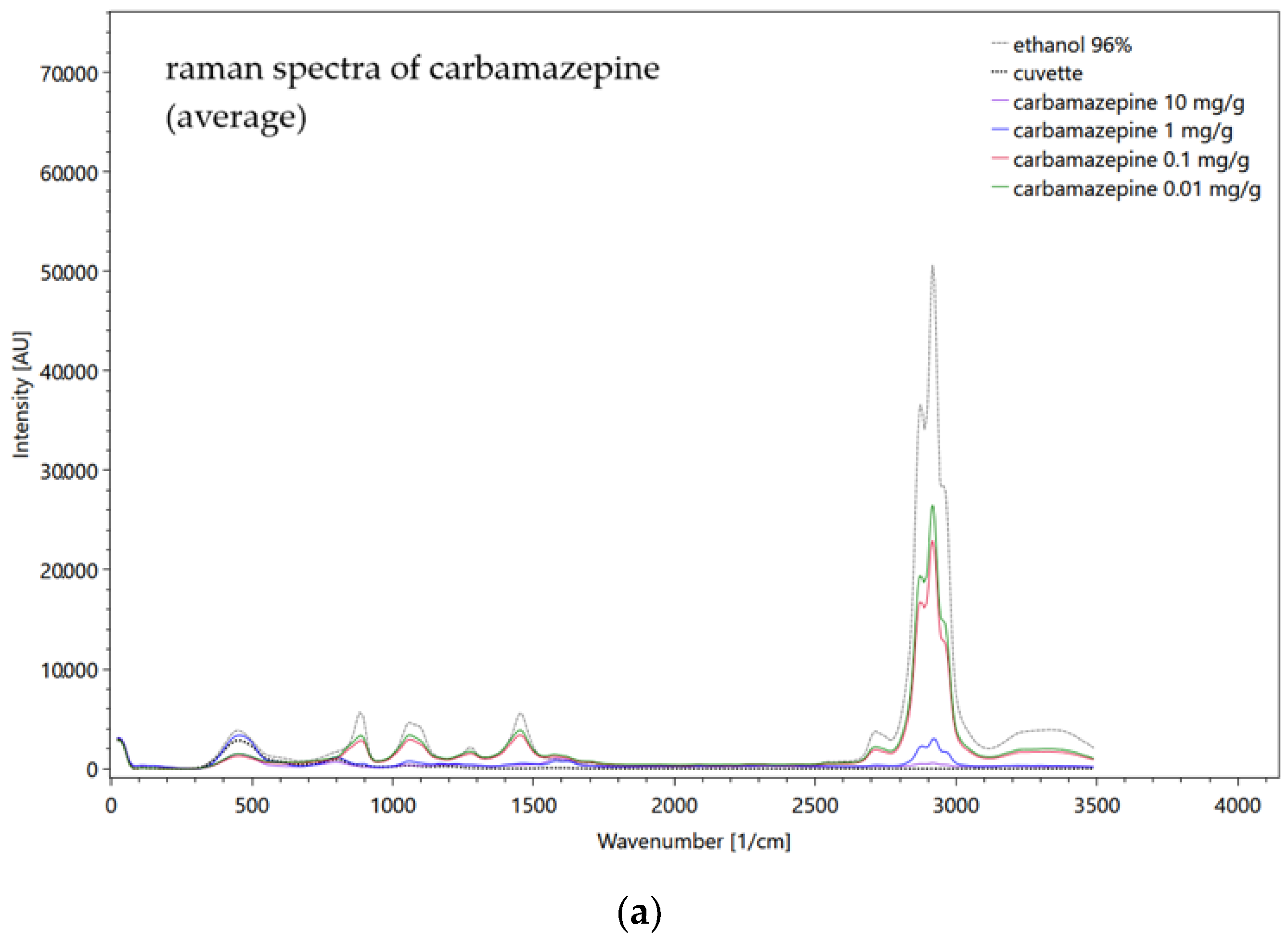
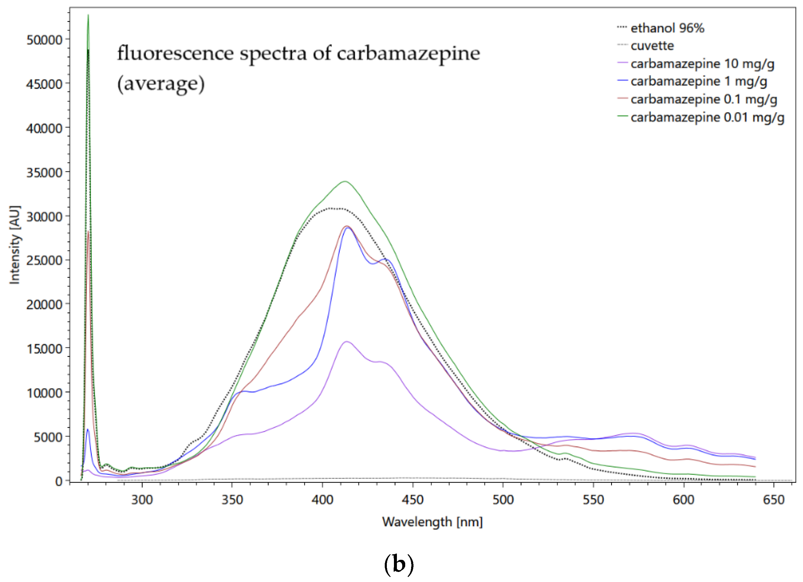
| Carbamazepine; 297-46-4; purity > 98% | BioTrend, Cologne, Germany | Pure powder in solution with cuvette from Starna Cells® Atascadero, CA, USA | Pure substance and 10; 1; 0.1; 0.01 mg/g in solution with ethanol | Preventive value 0.1 µg/L ° |
| Hydrochlorothiazide; 58-93-5; purity > 99% | BioTrend, Cologne, Germany | Pure powder in solution with cuvette from Starna Cells® Atascadero, CA, USA | Pure substance and 10; 1; 0.1; 0.01 mg/g in solution with ethanol | Preventive value 0.1 µg/L ° |
| Acetaminophen; 103-90-2; purity > 99% | BioTrend, Cologne, Germany | Pure powder in solution with cuvette from Starna Cells® Atascadero, CA, USA | Pure substance and 10; 1; 0.1; 0.01 mg/g in solution with ethanol | Preventive value 0.1 µg/L ° |
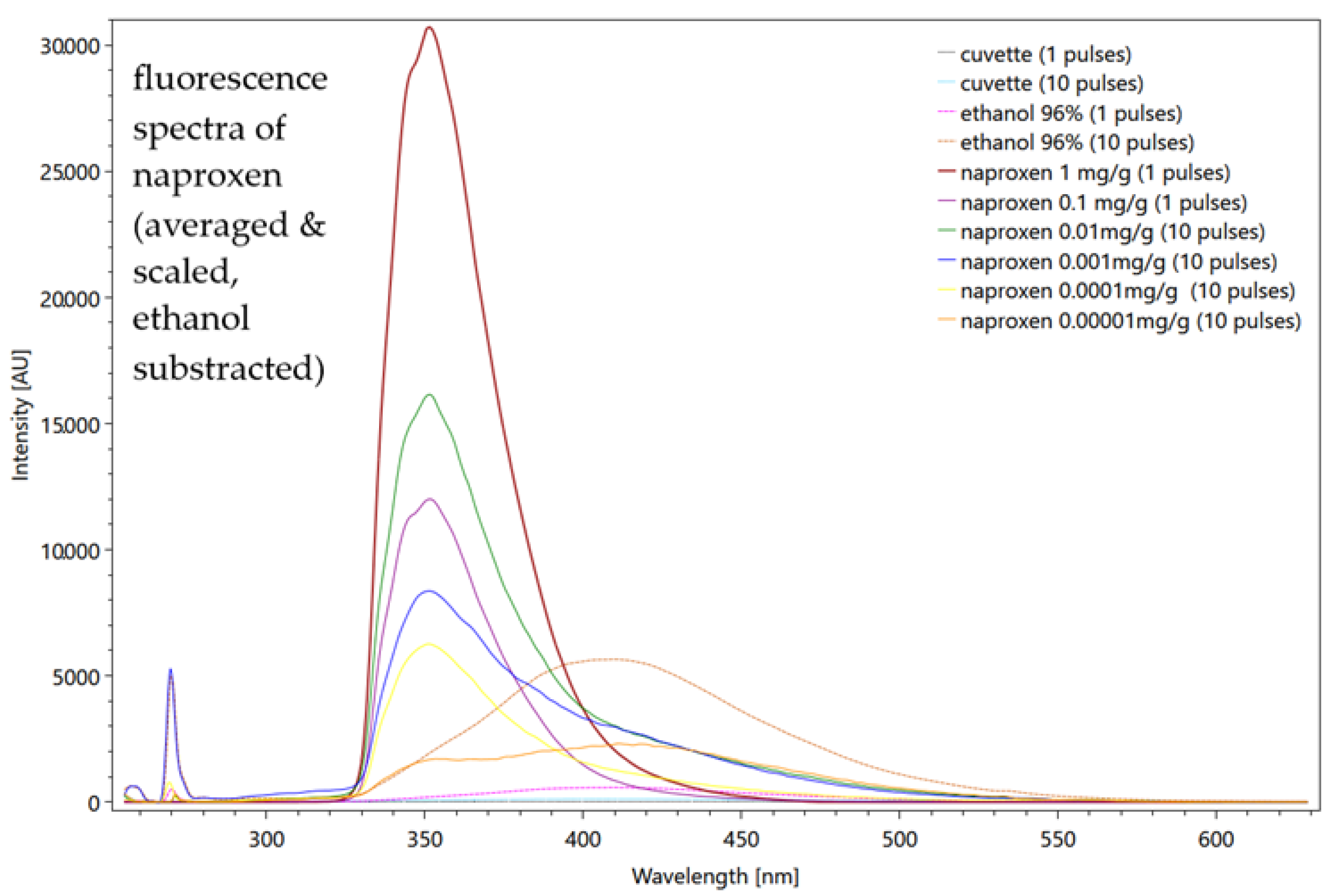
| Naproxen; 22204-53-1; purity > 98% | BioTrend, Cologne, Germany | Pure powder in solution with cuvette from Starna Cells® Atascadero, CA, USA | Pure substance and 0.005; 0.001; 0.0005; 0.00001 down to 1 × 10⁻⁵ mg/g in solution with ethanol | Preventive value 0.1 µg/L ° |
| Diclofenac; 15307-93-4; purity > 98% | BioTrend, Cologne, Germany | Pure powder in solution with cuvette from Starna Cells® Atascadero, CA, USA | Pure substance and 10; 5; 1; 0.5; 0.1; 0.05; 0.01 g/L in solution with Millipore®, Merck KGaA, Darmstadt, Germany | Water hazard class 3 + acc. to WDF watch list X |
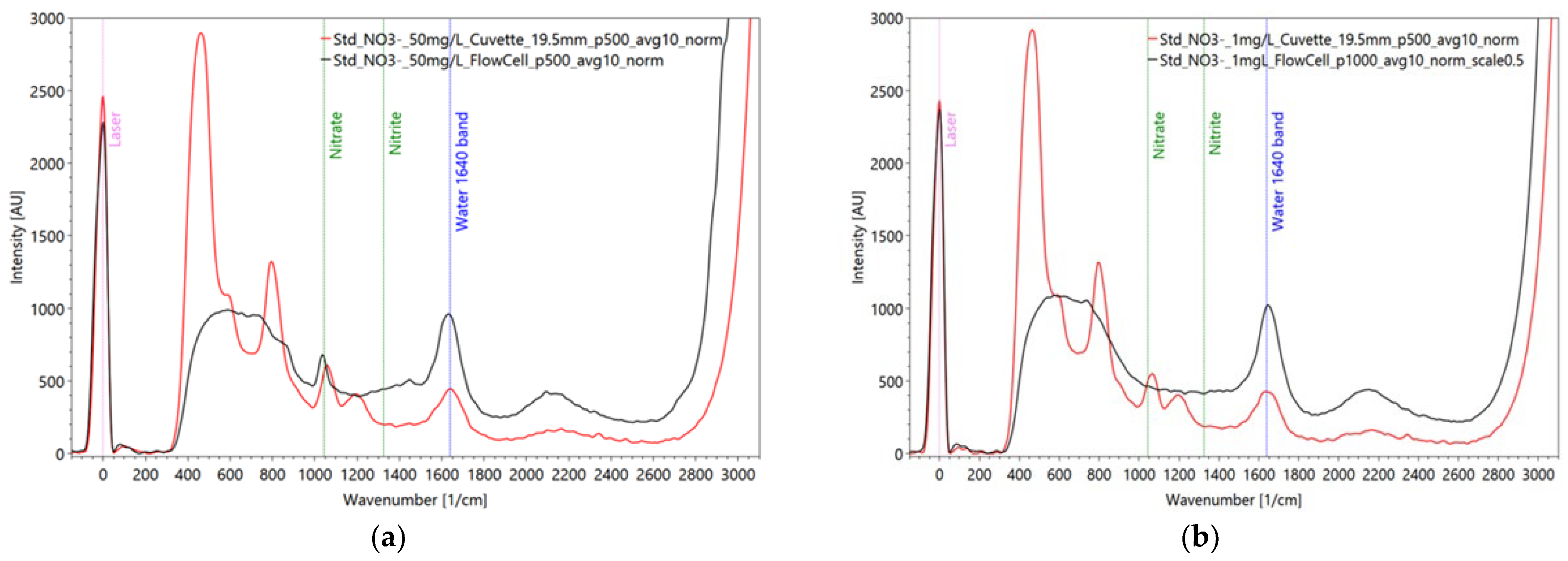
| Bromate; 7789-38-0 | VWR Chemicals | In solution with solvent water, in flow cell | 50; 25; 10; 5; 1; 0.1; 0.01 mg/L in solution with Millipore®, Merck KGaA, Darmstadt, Germany | 10 µg/L, according to Directive EU # |
| Bromide; 7647-15-6 | Supelco®, Merck KGaA, Darmstadt, Germany | In solution with solvent water, in flow cell | 50; 25; 10; 5; 1; 0.1; 0.01 mg/L in solution with Millipore® Merck KGaA, Darmstadt, Germany | - |
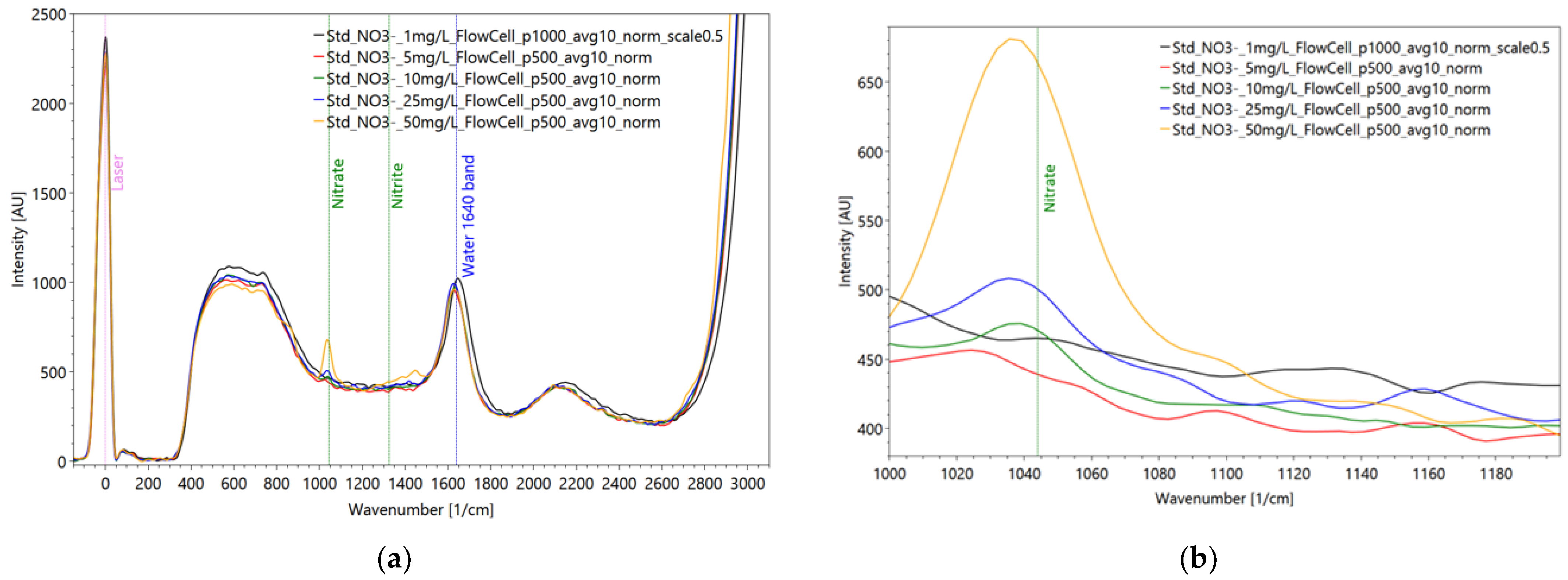
| Nitrate; 7631-99-4 | ROTI®Star Carl Roth GmbH + Co. KG, Karlsruhe, Germany | In solution with solvent water, in flow cell | 50; 25; 10; 5; 1 mg/L in solution with Millipore®, Merck KGaA, Darmstadt, Germany | 50 mg/L, according to WFD X and Directive EU # |
| Nitrite; 7632-00-0 | Certipur® Merck KGaA, Darmstadt, Germany | In solution with solvent water, in flow cell | 50; 25; 10; 5; 1 mg/L in solution with Millipore®, Merck KGaA, Darmstadt, Germany | 0.5 mg/L, according to Directive EU # |
| Tryptophan; 73-22-3 | Merck KGaA, Darmstadt, Germany | In solution and as a solid, cuvette from Starna Cells® | Pure substance and 10; 5; 1; 0.5; 0.1; 0.05 0.01; 0.005; 0.001 mg/L in solution with Millipore®, Merck KGaA, Darmstadt, Germany | - |
| Tyrosine; 60-18-4 | Carl Roth® Carl Roth GmbH + Co. KG, Karlsruhe, Germany | In solution and as a solid, cuvette from Starna Cells® | Pure substance and 10; 5; 1; 0.5; 0.1; 0.05 0.01; 0.005; 0.001 mg/L in solution with Millipore®, Merck KGaA, Darmstadt, Germany | - |
| Substance; CAS no. | Spectral Analysis | Detection | ||
|---|---|---|---|---|
| Raman | Fluorescence | Raman | Fluorescence | |
| Metformin hydrochloride; 1115-70-4; purity > 99% | ✓ | ✓ | - | - |
| Carbamazepine; 297-46-4; purity > 98% | ✓ | ✓ | ** | * |
| Hydrochlorothiazide; 58-93-5; purity > 99% | ✓ | ✓ | * | ** |
| Acetaminophen; 103-90-2; purity > 99% | ✓ | ✓ | ** | * |
| Naproxen; 22204-53-1; purity > 98% | ✓ | ✓ | *** | ** |
| Diclofenac; 15307-93-4; purity > 98% | ✓ | ✓ | - | - |
| Bromate; 7789-38-0 | ✓ | ✓ | - | ** |
| Bromide; 7647-15-6 | ✓ | ✓ | - | ** |
| Nitrate; 7631-99-4 | ✓ | ✓ | * | - |
| Nitrite; 7632-00-0 | ✓ | ✓ | * | - |
| Tryptophan; 73-22-3 | ✓ | ✓ | *** | *** |
| Tyrosine; 60-18-4 | ✓ | ✓ | *** | ** |
| DOC | ✕ | ✓ | - | ** |
Publisher’s Note: MDPI stays neutral with regard to jurisdictional claims in published maps and institutional affiliations. |
© 2022 by the authors. Licensee MDPI, Basel, Switzerland. This article is an open access article distributed under the terms and conditions of the Creative Commons Attribution (CC BY) license (https://creativecommons.org/licenses/by/4.0/).
Share and Cite
Post, C.; Heyden, N.; Reinartz, A.; Foerderer, A.; Bruelisauer, S.; Linnemann, V.; Hug, W.; Amann, F. Possibilities of Real Time Monitoring of Micropollutants in Wastewater Using Laser-Induced Raman & Fluorescence Spectroscopy (LIRFS) and Artificial Intelligence (AI). Sensors 2022, 22, 4668. https://doi.org/10.3390/s22134668
Post C, Heyden N, Reinartz A, Foerderer A, Bruelisauer S, Linnemann V, Hug W, Amann F. Possibilities of Real Time Monitoring of Micropollutants in Wastewater Using Laser-Induced Raman & Fluorescence Spectroscopy (LIRFS) and Artificial Intelligence (AI). Sensors. 2022; 22(13):4668. https://doi.org/10.3390/s22134668
Chicago/Turabian StylePost, Claudia, Niklas Heyden, André Reinartz, Aaron Foerderer, Simon Bruelisauer, Volker Linnemann, William Hug, and Florian Amann. 2022. "Possibilities of Real Time Monitoring of Micropollutants in Wastewater Using Laser-Induced Raman & Fluorescence Spectroscopy (LIRFS) and Artificial Intelligence (AI)" Sensors 22, no. 13: 4668. https://doi.org/10.3390/s22134668