Rapid Identification of Wood Species Based on Portable Near-Infrared Spectrometry and Chemometrics Methods
In this paper, a portable near-infrared (NIR) spectrometer, combined with chemometrics methods, was used for rapid identification of 20 wood species. Four spectral pretreatment methods, including Norris-Williams smooth (NWS), standard normal variate (SNV), multiplicative scatter correction (MSC) and Savitzky-Golay 1st derivative (SG 1st-Der), were adopted for noise reduction and information enhancement of near-infrared (NIR) spectra of wood. Three pattern recognition methods, including principal component analysis (PCA), partial least squares discriminant analysis (PLS-DA), and support vector machine (SVM), were used to cluster analysis of sample spectra. The competitive adaptive reweighted sampling (CARS) method was proposed to select effective wavelengths (EWs). The Bayesian information criteria (BIC) value was used for comprehensive evaluation of model accuracy and complexity. Compared with PLS-DA models, both the correction set and test set of the SG 1st-Der-SVM model and the SNV-SVM model have obtained 100% correct recognition rates (CRRs). The CARS method shows the SG 1st-Der-SVM model having the smallest BIC value, and the model was optimal.
Classification and identification of wood species is an important part of wood processing and trade. Different wood species have different physical or chemical properties, which is of great significance to entry-exit inspection, quarantine departments, and furniture enterprises. Conventional wood species identification methods include microscopic cell structure and surface characteristic analysis. The microscopic cell structure analysis method needs microscope and wood slices processing, and the analysis process is complex (1). The surface characteristic analysis method is mainly used to analyze the color and texture of wood surfaces by means of image and spectral analysis. Image analysis mainly includes image acquisition, image processing and image recognition, and the identification process requires expertise and is also complex (2). In the image acquisition stage, a high-resolution camera and light source are necessary to ensure the clarity of the image. Complex image pretreatment methods are needed to enhance and extract the image features. Image recognition needs a better template or model to ensure its accuracy.
In recent years, with the development of optical instruments, near-infrared (NIR) spectroscopy has been widely used in qualitative and quantitative analysis of physical and chemical properties of substances because of its fast, nondestructive, and simple operation. The NIR spectrum is electromagnetic energy with a wavelength range of 780–2500 nm. NIR spectra mainly detect overtones and combination bands of the substance; and different bonds, including C-O, O-H, C-H, S-H, and N-H, have different spectral absorption. NIR applications have increased in the agricultural and forest products industries (3,4). Thayna and associates used NIR and partial least squares (PLS) to predict total anthocyanins content (TAC) and total phenolic compounds (TPC) in intact wax jambu fruit (5). Chen and associates have used NIR and PLS to analysis main catechins contents in green tea (6). Luna and associates used NIR and multivariate classification to discriminate soybean oil samples into non-transgenic and transgenic types (7). Zhou and associates used NIR and chemometrics to separate a green hem-fir mix online (8).
The chemical composition of wood is very complex. Many experimental studies have shown that cellulose, hemicellulose, lignin, and other organic molecules (such as glucose, fructose, pinitol, sorbitol, and inositol) are contained in wood, and these substances all have spectral response in the NIR region (9–15).
In this paper, a portable NIR spectrometer combined with chemometrics methods is used for qualitative identification of 20 wood species. Different spectral pretreatment and pattern recognition methods are used to optimize the optimal recognition model, and predict attribution of an unknown wood species.
Materials and Methods
Samples
For this study, 20 wood species were collected from Zhang Jiagang Entry-Exit Inspection and Quarantine Bureau of China. There were 80 samples from 80 different trees per type of wood, and each sample was made with dimensions of 21 × 10 × 2 cm3 (length × width × height) according to the national standard method (16) for spectral collection and analysis. Therefore, a total of 1600 samples were used in the experiment.
To build the discriminant model and evaluate the accuracy of the model, 80 samples of each kind of wood were divided into calibration sets and test sets, with the ratio of 3:1 using the Kennard Stone (KS) method (17,18). Thus, a total of 1600 wood samples, of which 1200 samples were used to build the model and validation model, and the remaining 400 samples were taken as a test set for external test. To establish a multi-classification model, the 20 wood species were named 1 to 20 in sequence. The corresponding relationship between attribute values and wood species is shown in Table I.


NIR Spectra Acquisition
The NIR spectra were acquired by a portable spectrometer (MicroNIRS, VIAVI Corporation) with the spectral region of 900–1700 nm. The MicroNIRS instrument consists of a linear variable filter (LVF) dispersing element focused directly onto a 128-pixel linear indium gallium arsenide (InGaAs) array detector, and two tungsten light bulbs as the sources (19).
The NIR spectra acquisition system was set up based on a computer (with self-developed software based on Matlab R2014a) and the MicroNIRS spectrometer. For each wood sample, three diffuse reflectance spectra were measured randomly at different locations, with a temperature of 25±2 °C and humidity of 57±5% RH. Then, the mean spectrum of each wood sample is calculated and stored for the subsequent spectral analysis and species classification.
Traditional detection methods require multiple treatments of the wood, including cutting, softening, slicing, dyeing, dehydrating, and transparency processing. Pictures of the processed wood samples are then taken, or the samples may be observed through a microscope, and the characteristics and microstructure of the wood samples are compared with the standard wood to determine the type of wood being studied. The proposed wood type identification system is only required to collect the spectrum of the wood, and determine the type of wood by using chemometric analysis.
Methods
NIR spectra are often accompanied by noise for some factors, mainly because of the instability of the light source or detector due to temperature and power supply fluctuations, spectral acquisition modes and sample state variations, and other factors. Therefore, spectral pretreatment is very important for NIR analysis. Four spectral pretreatment methods, including Norris-Williams smooth (NWS) (20), standard normal variate (SNV) (21), multiplicative scatter correction (MSC) (22) and Savitzky-Golay 1st derivative (SG 1st-Der) (23), are used for noise reduction and information enhancement of the NIR wood spectra.
The NIR spectra are highly overlapping, so it is necessary to use chemometrics methods, such as principal component analysis (PCA), partial least squares discriminant analysis (PLS–DA) and support vector machines (SVM), for spectral interpretation. PCA is a method for dimensionality reduction for high-dimensional data by decomposing linear combination of origin variables into a few principal components (24,25). PCA was used to observe the samples spectral spatial distribution. PLS–DA and SVM are used to build discriminant models.
For the PLS–DA method, the latent variable (LV) is an important optimization parameter (26,27), and a reasonable number of LV can make full use of spectral information and filter out noise (28). The Monte Carlo cross-validation (MCCV) method, proposed by Picard and Cook (29), is used to determine the number of LV. MCCV is a simple and effective method that can reduce the risk of model overfitting. The repeated MCCV criterion is defined in equation 1. When the MCCV is the smallest, the m is the number of LV:


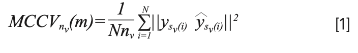
where y and ŷ are the true and predicted values of the samples, nv is the size of the test sample, and repeat the procedure N times (i = 1, 2, ..., N).
SVM is based on the statistical learning theory and structural risk minimization. The basic principle of SVM is to find the optimal separation hyperplane to make the classification problem linearly separable (30). Assuming a sample set:


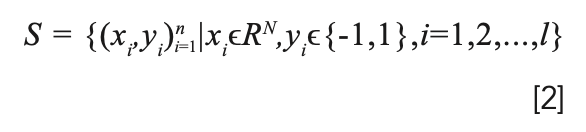
Among them, xi is the sample data, and yi is the sample category. The optimization problem is written as:


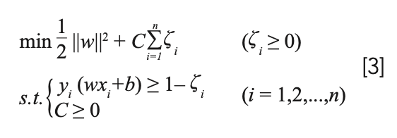
where w represents the weight vector and b represents the bias vector. C is the penalized regression error. In order to ensure the accuracy of classification, introduce a relaxation factor


As the classifier is a linear function, it is necessary to ensure that the classification hyperplane can accurately distinguish the two types of samples while also ensuring the maximum classification interval. For the case where the classifier is a nonlinear function, it is necessary to map the nonlinear separable problem in the low-dimensional space to the high-dimensional space by introducing the kernel function, and then find the optimal classification hyperplane in the high-dimensional space.
The radial basis function (RBF) is used as the kernel function, and expression of RBF is shown in equation 4 (31). Two parameters, penalized regression error (C) and gamma (g), need to be optimized to get the best analysis model, and the grid search (GS) method is employed to select optimal C and g. The expression of g is shown in equation 5:


where xi is the training sample, x is the sample to be predicted, and σ is the width of the kernel function.
Competitive adaptive reweighted sampling (CARS) is a characteristic wavelength selection method based on Monte Carlo sampling and PLS regression coefficients (32). It can overcome the combinatorial explosion problem in variable selection to a certain extent, filter out an optimized subset of variables, and improve the predictive ability of the model. Establish the corresponding PLS model through the correction set samples selected by Monte Carlo sampling, and calculate the weight of the absolute value of the wavelength regression coefficient in this sampling. The larger the weight value, the greater the contribution of the variable to the establishment of the model. Remove the wavelength variables with small absolute values, and the number of variables is determined by the exponential decay function (EDF) (33). The remaining wavelength variables adopt adaptive reweighted sampling to select multiple subsets of wavelength variables to establish a PLS model. The subset of the model with the smallest root mean square error of cross-validation (RM-SECV) is the selection of characteristic wavelength combinations. The calculation process is as follows:


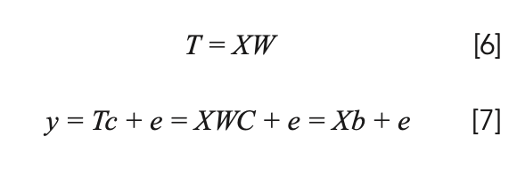
where X is the spectral data of the sample and y is the attribute value of each sample. T is the score matrix of X, which is a linear combination of X and W; c is the regression coefficient vector of y against T by least squares; and e is the prediction error. The method used in the paper was run under Matlab R2014a.
Model Evaluation
The correct recognition rate (CRR) is used to evaluate the accuracy of the model. Good models have relatively higher CRR. The formula is as follows:


where p represents the number of correctly identified samples, and t represents the total number of samples.
To compare the best performing models, the Bayesian information criteria (BIC) (34) is used to determine a satisfactory compromise between model accuracy and model simplicity. The calculation formula of BIC is shown in equation 9:


In the formula, CRR is the accuracy of the model, n is the number of samples, and k is the number of variables to build the model. The model with the minimum BIC is optimal.
Results and Discussion
NIR Spectra of Wood Samples
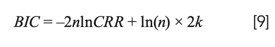
Figure 1 shows the NIR spectra of a total of 200 wood samples randomly selected —10 samples from each type of wood. The absorbance spectra range was from 0.6 to 2.2 AU. The absorption peak appears at a wavelength of 1100 nm; this is because of the in-plane bending vibration of the aromatic C-H and the tensile vibration of the secondary alcohol C-O in the wood. Each spectrum is smooth, and the contour trends are consistent. However, when multiple wood spectra are plotted together, the spectra are interlaced and cannot be resolved intuitively. Further preprocessing and pattern recognition methods are required for spectral analysis.


FIGURE 1: NIR absorbance spectra of wood samples.
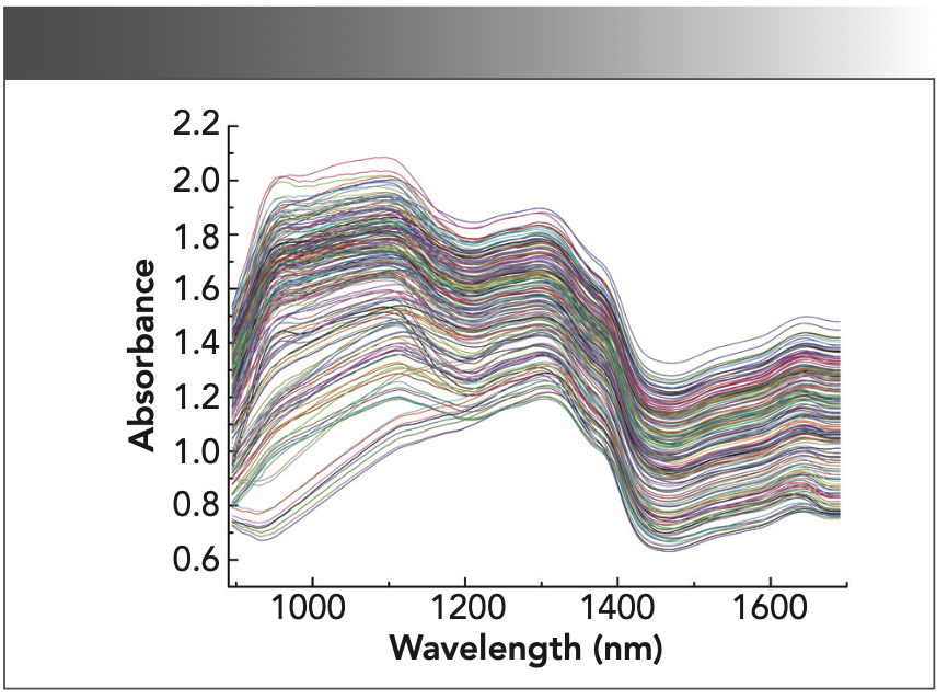
Figure 2 shows the NIR spectra of wood samples employing the different pretreatment methods, including NWS, SNV, MSC, and SG 1st-Der. Different woods show different spectral characteristics after spectral pretreatment due to the fact that NIR spectra signature is strongly affected by the growth environmental conditions and texture of wood (35). Nevertheless, it is not possible to observe significant visual differences between the spectra.

 NWS, (b) SNV, (c) MSC, and (d) SG 1st-derivative.")
FIGURE 2: The NIR spectra of wood samples employing the different pretreatment methods: (a) NWS, (b) SNV, (c) MSC, and (d) SG 1st-derivative.

PCA Result of Wood Species
PCA was applied to find the characteristics of each wood species according to the 1600 original spectra. Every wood has many characteristics that can be measured in spectra. PCA can select the important characteristics that can classify them among the 20 species of wood according the spectra, and reduce dimensionality based on decomposing linear combination of origin variables into a few principal components (36).
The distribution diagram of the first three principal components of the calibration wood samples is shown in Figure 3. The cumulative contribution rate of the first three principal components reached 99.8%. In Figure 3, we use different colored points to represent 20 types of wood, and there are 80 samples of each kind of wood. As shown in the figure, the sample points representing different wood species are interlaced with each other. It can be also be seen in the figure that PCA cannot clearly classify the 20 wood species in the form of a simple classification plane.


FIGURE 3: The distribution diagram of the first three principal components of the calibration set wood samples.
PLS–DA Model Analysis of Wood Species
PLS–DA models for identification of wood species were developed with origin and preprocessing spectra. MCCV was used to select the optimal number of LVs. For the MCCV method, 1200 samples were used for random sampling modeling, and 840 were selected for modeling each time, with the remaining 360 used for model verification. The number of random cycles was set to 500, and the model was evaluated using the CRR. The ordinate of Figure 4 is the average of CRR of 500 cycles. For origin spectra PLS–DA model, when LVs are 17, the curves of CRR tend to be flat, and the standard deviation (SD) of 500 operations is small for calibration and test sets. There is no risk of overfitting for models with approximately equal value of CRRs for both calibration and test sets. The results of classification for wood species based on PLS–DA models with origin and preprocessing spectra are shown in Table II, where it can be seen that the origin spectra PLS–DA model was optimal with 17 LVs, and the CRRs were 97.50% and 98.25% for calibration and test sets, respectively.


FIGURE 4: The trend chart of CRR changing with LVs in the calibration and test set.


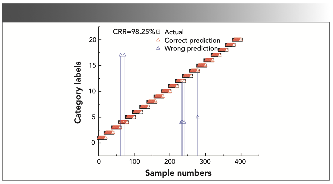
Figure 5 shows the scatter plot of the real attribute value and the predicted value of the origin spectra PLS–DA model for test set samples. The square and triangle represent the true attribute values of the test set and predictive attribute values of the optimal PLS–DA model, respectively. The coincidence degree of square and triangle reflects the precision of the model. The higher the coincidence degree in the scatter plot, the better the prediction accuracy of the model; the red triangle represents the correct prediction, and the blue triangle represents the wrong prediction. As shown in Table II, the value of CRR was 98.25%. It clearly observed that seven samples showed incorrect validation results in Figure 5. Among them, two samples of No. 4 (Aglaia spp) wood were wrongly predicted to be No. 17 (Khaya spp) sample, four samples of No. 12 (Canarium spp) wood were wrongly predicted to be No. 4 sample, and one sample of No. 14 (Mansonia altissima) wood was wrongly predicted to be No. 5 (Burckella spp) sample. As to reasons behind the wrong prediction of wood, a possible reason is that the absorption of the double frequency and the combined frequency of the hydrogen-containing groups of the two woods is similar.


FIGURE 5: The scatter plot of the real attribute value and the predicted value of PLS-DA model for test set samples.
SVM Model Analysis of Wood Species
The regularization constant C and the kernel function parameter g are the key parameters that affect the performance of the SVM. The basic idea of the GS method is an exhaustively search for optimization parameters; arrange and combine the possible values of each parameter, list all possible combinations to generate grid, and then each combination is brought into the model to verify its performance. Finally, the parameter values that make the model performance optimal are taken as the best parameters.
SVM models were developed with origin and pretreated spectra. Table III summarizes the modeling results. From Table III, it is possible to observe that SG 1st-Der and SNV pretreatment promoted the best SVM model, with 100% CRR for calibration set and test set. According to the prediction accuracy, the prediction result of the SVM model was better than the PLS–DA model, proving that the kernel introduced by SVM was a good predictor of the nonlinear relationship between spectral data and wood species.


Establishment of CARS–SVM Model
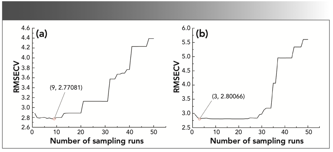
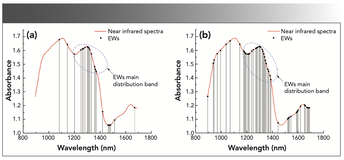
To build a more parsimous discriminant model, a CARS (37,38) method was proposed to remove redundant variables with collinearity and select effective wavelengths. The number of repeated sampling of the CARS method was set to 50, and the five-fold cross-validation method was used to calculate the RMSECV. At the beginning of the EDF, as the number of sampling variables was eliminated, the RMSECV decreased, and then the number of sampling iterations continued to increase rapidly because of the decrease of effective wavelengths (EWs). At the end, interactive verification was used to select the smallest subset of RMSECV as the optimal variable combination. It can be concluded in Figure 6 that, when the number of sampling runs of the SG 1st-Der-CARS–SVM model was 9, the RMSECV reaches the minimum (Figure 6a), and 22 EWs were selected. When the number of sampling runs of the SNV–CARS–SVM model was 9, the RMSECV reaches the minimum (Figure 6b), and 48 EWs were selected. Figure 7a was the distribution map of 22 EWs selected by the SG 1st-Der-CARS–SVM model, and Figure 7b was the distribution map of the 48 EWs selected by the SNV–CARS–SVM model. The red line represents a spectrum, and the black circle represents EWs. From the figure, EWs are mainly distributed between 1200–1400 nm (The point inside the blue circle in Figure 7). In this band, the spectrometer introduces the least external interference in the process of collecting spectral data, and contains the most effective data.

 the model of SG 1st-Der-CARS-SVM; and (b) the model of SNV-CARS-SVM.")
FIGURE 6: The relationship between RMSECV and the number of sampling runs in the CARS method; (a) the model of SG 1st-Der-CARS-SVM; and (b) the model of SNV-CARS-SVM.

 The model of SG 1st-Der-CARS-SVM selected 22 EWs; (b) The model of SNV-CARS-SVM selected 48 EWs.")
FIGURE 7: Distribution map of EWs selected by CARS; (a) The model of SG 1st-Der-CARS-SVM selected 22 EWs; (b) The model of SNV-CARS-SVM selected 48 EWs.
In the process of establishing a discriminant model, choosing different combinations of variables would result in different models, and the values corresponding to the information criteria would also change. In this study, the calibration set and test set CRR of the SG 1st-Der-CARS–SVM model were both 100% (Table IV), but the variable combinations of the two models were different. Therefore, the corresponding BIC was not the same. As shown in Table IV, it can be concluded that the BIC value of the calibration set and the test set of the SG 1st-Der-CARS–SVM model were the smallest. The SG-1st-Der-CARS–SVM model used fewer variables for modeling. While ensuring the accuracy of model prediction, the model was simplified to make the model better.


Conclusion
In this study, 20 wood species were classified successfully based on the portable NIR spectra with chemometrics methods of PLS–DA and SVM. Compared to PLS–DA, the SG 1st-Der-SVM model and the SNV–SVM model both obtained 100% CRRs in the calibration set and test set for classifying 20 kinds of wood. The CARS method can effectively filter out EWs, reduce the invalid variables in the modeling, and simplify the SVM model. By comparing the calculated value of the models, the BIC value of the SG 1st-Der-CARS–SVM model was the smallest. The results show that the SG 1st-Der-CARS–SVM model is the best. A portable NIR spectrometer combined with SVM method can be used for fast identification of wood species with a higher recognition rate.
Conflicts of Interest
The authors declare no conflict of interest.
Acknowledgments
This work was supported by National Natural Science Foundation of China (21265006).
References
(1) G. Dou, G.S. Chen, and P. Zhao, Spectrosc. Spectral Anal. 36(8), 2425–2429 (2016). Doi: 10.3964/j.issn.1000-0593(2016)08-2425-05
(2) K.P. Cui, X.R. Zhai, and H.J. Wang, Advances in Forestry Letters 2(4), 61–66 (2013).
(3) Z.Y. Liu, F. Xu, J.B. Wen, and H.Z. Chen, Chinese J. Anal. Lab. 35(10), 1117–1120 (2016).
(4) Y.N. Liu, Z. Yang, B. Lu, M.M. Zhang, and X.H. Wang, Spectrosc. Spectral Anal. 34(3), 648–651 (2014).
(5) T.R. Viegas, A.L.M.L. Mata, M.M.L. Duarte, and K.M.G. Lima, Food Chem. 190(1), 1–4 (2016). Doi: 10.1016/j.foodchem.2015.05.063.
(6) Q.S. Chen, J.W. Zhao, C. Sumpun, and Z.M. Guo, Food Chem. 113(4), 1272–1277 (2009). Doi: 10.1016/j.foodchem.2008.08.042
(7) A.S. Luna, A.P. da Silva, J.S.A. Conclusion Pinho, J. Feree, and R. Boque, Spectrochim. Acta A 100, 115–119 (2013).
(8) Z. Zhou, S. Sohrab, and S. Avramidis, Eur. J. Wood Wood Prod. 78(1), 151–160 (2020). Doi: 10.1007/s00107-019-01479-8
(9) E. Pecoraro, B. Pizzo, A. Alves, N. Macchioni, and J.C. Rodrigues, Microchem. J. 122, 176–188 (2015).
(10) C.J.G. Colares, T.C.M. Pastore, V.T.R. Coradin, L.F. Marques, A.C.O. Moreira et al., Microchem. J. 124, 356–363 (2016). Doi: 10.1016/j.microc.2015.09.022
(11) A. Sandak, J. Sandak, and M. Zborowska, J. Archaeol Sci. 37(9), 2093–2101 (2010). Doi: 10.1016/j.jas.2010.02.005
(12) L. Tong and W.B. Zhang, Appl. Spectrosc. 70(10), 1676–1684 (2016). Doi: 10.1177/0003702816644453
(13) X.S. Wang, Y.D. Sun, and M.G. Huang, J. Northeast Forestry University 43(12), 82–85 (2015).
(14) B. Pizzo, E. Pecoraro, and N. Macchioni, Appl. Spectrosc. 67(5), 553–562 (2013). Doi: 10.1366/12-06819
(15) K. Zhao, Y. Xiong, and M. Zhao, Laser & Infrared 41(6), 649–652 (2011).
(16) National Timber Standardization Technical Committee, General Method of Wood Identification: GB/T 29894-2013 (Standards Press of China, Beijing, People’s Republic of China, 2013), pp. 1–12.
(17) H. Li, J.X. Wang, Z.N. Xing, and G. Shen, Spectrosc. Spectral Anal. 31(2), 362–365 (2011). Doi: 10.3964/j.issn.1000-0593(2011)02-0362-04
(18) W. Liu, Z. Zhao, H.F. Yuan, C.F. Song, and X.Y. Li, Spectrosc. Spectral Anal. 34(4), 947–951 (2014). Doi: 10.3964/j.issn.1000-0593(2014)04-0947-05
(19) K.N. Basri, M.N. Hussain, J. Bakar, Z. Sharif, and M.F.A. Khir, Spectrochim Acta A 173, 335–342 (2017).
(20) M. Asachi, A. Hassanpour, and M. Ghadiri, et al., Powder Technol. 320, 143–154 (2017).
(21) R.J. Barnes, M.S. Dhanoa, and S.J. Lister, Appl. Spectrosc. 43(5), 772–777 (2016).
(22) Q.X. Zhang, Q.B. Li, and G.G. Zhang, Spectroscopy 26(7), 28–39 (2011).
(23) P.Y. Diwu, X.H. Bian, Z.F. Wang, and W. Liu, Spectrosc. Spectral Anal. 39(9), 2800–2806 (2018).
(24) V.K. Keerthi and B. Surendiran, Perspectives in Science 8(C), 510–512 (2016). Doi: 10.1016/j.pisc.2016.05.010
(25) Y.F. Wang, X.D. Ma, and J.J Malcolm, Renew Energ. 97, 444–456 (2016). Doi: 10.1016/j.renene.2016.06.006
(26) K.H. Wong, N.V. Razmovski, K.M. Li, G.Q. Li, and K. Chan, J. Pharmaceut. Biomed. 84, 5–13 (2013). Doi: 10.1016/j.jpba.2013.05.040
(27) L. Sthle and S. Wold, J. Chemomet. 1(3), 185–196 (1987). Doi: 10.1002/cem.1180010306
(28) M. Barker, and W. Rayens, J. Chemomet. 17(3), 166–173 (2003). Doi: 10.1002/ cem.785
(29) Q.S. Xu and Y.Z. Liang, Chemomet. Intell Lab. 56(1), 1–11 (2001). Doi: 10.1016/S0169-7439(00)00122-2
(30) C. Cortes and V. Vapnik, Machine Learning 20(3), 273-297 (1995). Doi: 10.1007/ BF00994018
(31) J. Kivinen, A.J. Smola, and R.C. Williamson, IEEE T. Signal Proces. 52(8), 2165–2176 (2004). Doi: 10.1109/TSP.2004.830991
(32) J.B. Li, Y.K. Peng, L.P. Chen, and W.Q Huang, Spectrosc. Spectral Anal. 34(5), 1264–1269 (2014).
(33) K.Y. Zheng, T. Feng, W. Zhang, and X.W Huang, et al., Chemometr Intell Lab. 191, 109–117 (2019).
(34) S. Hiroshi, N. Kenji, Y. Hideki, M. YohIchi, and S. Hayaru, Sci. Technol. Adv. Mat. 21(1), 402-419 (2020). Doi: 10.1080/14686996.2020.1773210
(35) F. Guo, and M.A. Clemens, Spectrochim. Acta A 211, 254–259 (2019). Doi:10.1016/j.saa.2018.12.012
(36) C.H. Liu, X.H. Lu, and H.Y. Fan, Environ. Sci. Manag. 36(3), 183–186 (2011)
(37) E. Bonah, X.Y. Huang, R. Yi, J.H. Aheto, and S.H. Yu, Infrared Phys. Tech. 105, (2020). Doi: 10.1016/j.infrared.2020.103220
(38) J. Hui, W.D. Xu, Y.H. Ding, and Q.S. Chen, Spectrochim. Acta A 228 (2019). Doi: 10.1016/j.saa.2019.117781
Yong Hao and Qiming Wang are with the School of Mechatronics and Vehicle Engineering, at East China JiaoTong University, in Nanchang, China. Shumin Zhang is with the Technology Center of Nanchang Customs District, in Nanchang, China. Direct correspondence to: haonm@163.com ●