
Air Quality Measurements in Kitchener, Ontario, Canada Using Multisensor Mini Monitoring Stations
by

Wisam Mohammed
1, 
Nicole Shantz
1,
Lucas Neil
2,
Tom Townend
3,
Adrian Adamescu
1 and
Hind A. Al-Abadleh
1,* 1
Department of Chemistry and Biochemistry, Wilfrid Laurier University, Waterloo, ON N2L 3C5, Canada
2
Hemmera Envirochem Inc., Burlington, ON L7L 6B8, Canada
3
AQMesh, Environmental Instruments Ltd., Unit 5, The Mansley Centre, Timothy’s Bridge Road, Stratford-upon-Avon CV37 9NQ, UK
*
Author to whom correspondence should be addressed.
Atmosphere 2022, 13(1), 83; https://doi.org/10.3390/atmos13010083
Submission received: 30 November 2021
/
Revised: 21 December 2021
/
Accepted: 22 December 2021
/
Published: 5 January 2022
(This article belongs to the Special Issue High-Resolution Measurements of Atmospheric Pollutants, Pushing the Limit of Temporal and Spatial Resolution)
Abstract
:The Region of Waterloo is the third fastest growing region in Southern Ontario in Canada with a population of 619,000 as of 2019. However, only one air quality monitoring station, located in a city park in Kitchener, Ontario, is currently being used to assess the air quality of the region. In September 2020, a network of AQMesh Multisensor Mini Monitoring Stations (pods) were installed near elementary schools in Kitchener located near different types of emission source. Data analysis using a custom-made long-distance scaling software showed that the levels of nitrogen oxides (NO and NO2), ground level ozone (O3), and fine particulate matter (PM2.5) were traffic related. These pollutants were used to calculate the Air Quality Health Index-Plus (AQHI+) at each location, highlighting the inability of the provincial air quality monitoring station to detect hotspot areas in the city. The case study presented here quantified the impact of the 2021 summer wildfires on the local air quality at a high time resolution (15-min). The findings in this article show that these multisensor pods are a viable alternative to expensive research-grade equipment. The results highlight the need for networks of local scale air quality measurements, particularly in fast-growing cities in Canada.

1. Introduction
Pollutant emissions in urban communities remain a major concern among government bodies worldwide. The World Health Organization (WHO) reports that approximately 4.2 million deaths annually from around the world are directly linked to poor air quality exposure [1]. In 2016, the United Nations Children’s Fund (UNICEF) reported 600,000 deaths among youths globally as a result of prolonged exposure to polluted air causing lower respiratory infections [2]. These pollutants include nitric oxide (NO), nitrogen dioxide (NO2), ground level ozone (O3), and fine particulate matter (PM2.5). Although the main sources of pollutant emissions vary across regions globally, NO emissions mainly originate from the combustion of fossil fuels [3,4,5]. Fine particulate matter with sizes of 2.5 microns and smaller (PM2.5) are emitted from natural sources such as wind-blown mineral dust particles and sea spray from oceans [6]. Anthropogenic sources of PM2.5 in urban environments are emitted from transportation and industrial plants. Volatile organic compounds emitted from natural and anthropogenic sources play a role in complex atmospheric reactions leading to the production of PM2.5 in the form of secondary organic aerosol (SOA) [4,6].
In 1970, the amendment to the Clean Air Act (The Act) was legislatively passed in both Canada and the United States with additional revisions taking place over the following years [7]. The Act aimed to greatly reduce emissions from vehicles and manufacturing and mitigate the long-term impacts of acid rain and poor air quality [4,7,8]. The Act also incorporated many regulations focused on industry that have been gradually tightened over the past 50 years through a series of revisions in an effort to minimize emission levels of total suspended particles (TSPs) [7]. As a result of the implementation of these updated regulations, the exposure limits for numerous ambient pollutants were established, resulting in significantly reduced frequency of smog and acid rain events [8]. Table 1 lists the most recent short-term (1 h, 8 h, 24 h) exposure limits detailed in the Ontario Ambient Air Quality Criteria (AAQC) [9] in comparison with the recently released WHO Air Quality Guidelines (AQG) [10].
Indicator pollutants of air quality in Ontario are monitored by a network of 39 stations across the province maintained by the Ministry of the Environment, Conservation and Parks (MECP) [4]. One of these stations is located in Kitchener, Ontario, the largest city in the Region of Waterloo, which is also home to the cities of Cambridge and Waterloo among four other townships. The Waterloo Region is a thriving community with a growing population of 619,000 as of 2019. This region is also the third largest growing region in Canada according to Statistics Canada, after Oshawa and Halifax [11]. The long-term Climate Action Strategy for the Waterloo Region is to reduce Greenhouse Gas (GHG) emissions by 80% relative to 2010 by the year 2050 [12]. With an increasing population and development in the region, installation of air quality and greenhouse gas monitoring networks would be valuable to identify emission sources at local scales to better inform policies and initiatives aimed at improving air quality and reducing GHG emissions.
For comparison, in July of 2018, the Breathe London Blueprint project was launched in London, UK, which aimed at providing a hyperlocal air quality monitoring network with a real time map of ambient pollution across the city [13]. This project was the largest air quality monitoring network launched to date and consisted of over 100 multisensor pods developed by AQMesh and deployed across the city. The results from this network showed that approximately 90% of their stations detected very poor air quality [13]. This project not only allowed for the characterization of these highly polluted areas, but also provided insights into the source(s) of pollutants. The data collected were compelling regarding the need to reduce pollutant emissions in the city over decades of gradual change. This project inspired France, China, and the United States to launch similar air quality monitoring networks in their highly polluted regions [14,15].
Using the Breathe London Blueprint as a guide, our pilot study, which consisted of installing five multisensor AQMesh pods across Kitchener was launched in September 2020. The focus of this study was to measure pollutant levels near four elementary schools in Kitchener where children are classified as the “at-risk” group. Measurements were made before, during, and after the COVID-19 lockdown restrictions (See Supplemental Table S1). The global pandemic began in March 2020, six months after the multisensor pod network was installed. As a result, the AQMesh network had data collected prior to the global pandemic, during all lockdown restrictions that took place, and during the reopening phases of the province (See Supplementary Table S1).
The goal of this study was to analyze data from multisensor pods in a suburban environment with a strong emphasis on the comparisons between time periods when parents drop off students at school (7:00–10:00 a.m. Standard Eastern Time) and pickup at the end of school (3:00–6:00 p.m. Standard Eastern Time) during the work week. We also present a case study on the impacts of the 2021 wildfires in northern Ontario on the local air quality in Kitchener.
2. Materials and Methods
2.1. Spatial Location of the AQMesh Multisensor Pods
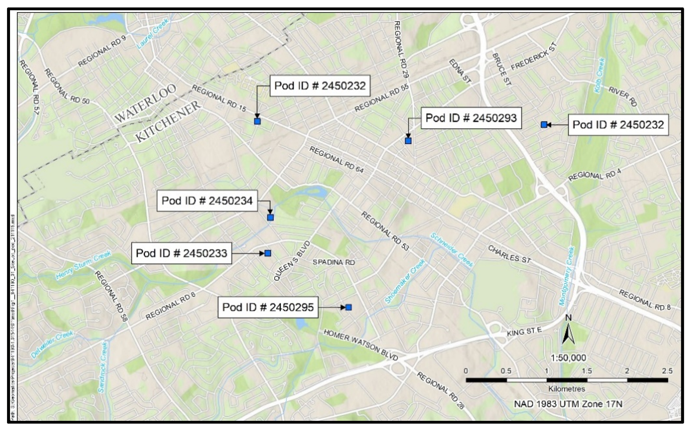
Five multisensor pods [16] (model version 2020) developed by AQMesh were installed in Kitchener, ON. Four sensor pods are located in close proximity to elementary schools. The fifth sensor pod (Pod 2450234) is co-located within 30 m of the MECP air quality reference monitoring station in Victoria Park (hereafter, “Reference Station”). The four multisensor pods installed outside the elementary schools were distributed between 500 m and 2 km from the reference station to capture a range of potential pollutant characteristics. Each multisensor pod detects pollutants at a high time resolution of 15 min and is equipped with electrochemical sensors that measure NO, NO2, O3, and CO, a Non-Dispersive Infrared (NDIR) sensor that measures CO2, and light scattering optical particle counters that measure particulate matter concentrations at PM1, PM2.5, PM4, and PM10 [17]. Figure 1 shows a map with the location of the multisensor pods. Table 2 highlights the Universal Transverse Mercator (UTM) coordinates of each pod along with the nearby respective elementary school.
2.2. Analysis of Co-Located Multisensor Pod Performance in Relation to the Reference Station
The AQMesh long distance scaling tool allows for comparisons between the monitoring points which are beyond the normal co-location distance (less than 1 m). This is achieved by separating the hyper local pollution events from regional responses by the sensor network. Then, as any differences in the instrument responses to each pollutant should be due to these hyper local events and as all instruments respond to regional pollution levels, comparison and scaling can be completed using only the regional pollution response.
Regional pollution response is determined by comparison of all AQMesh pods within the network. Hyper local events for individual pods are identified and temporarily redacted from the data set using a variation of the Grubbs method which identifies outliers within a data set. Once the regional data set for each pod is separated, it is compared to the regional data set from a reference station within the bounds of the AQMesh network. Criteria as specified by the US EPA for small sensor targets during co-location are then expected to be met [18]. While these targets are only currently published for O3 and PM2.5, similar expectations for R2, bias (slope and offset) and accuracy (RMSE) should be met for all other sensor species. Once slope and offset values are found using the regional data set for each pod, as linearity of response from the sensor is expected across the full range, these scaling values can be applied to the whole PreScaled data set which includes both hyper local and regional responses.
3. Results and Discussion
3.1. Performance Comparison with the Reference Station
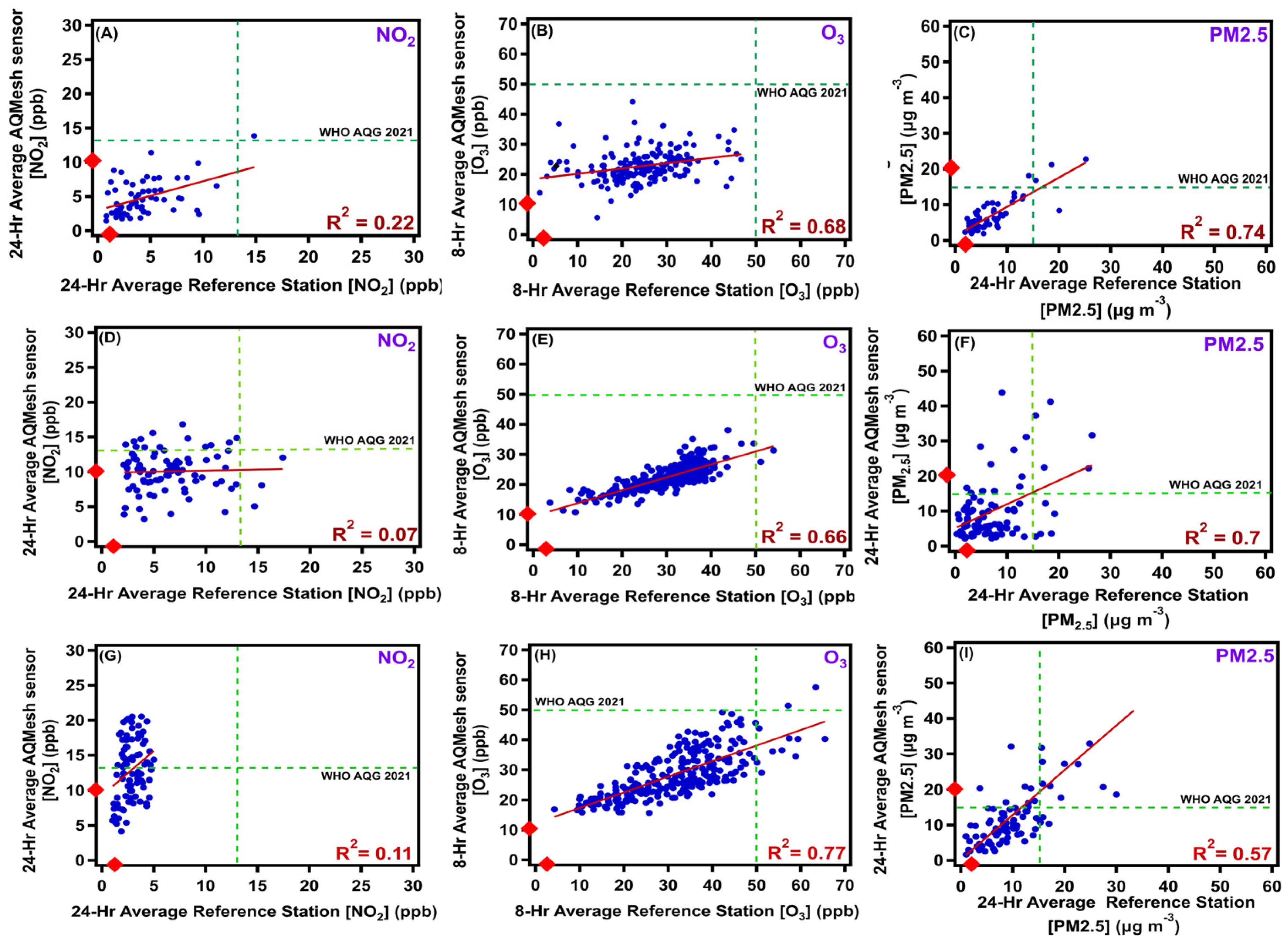
Supplementary Table S2 lists the limit of confidence (LOC) for both the AQMesh sensors per pollutant, and the reference station. Evidently, the AQMesh sensor pods have a larger LOC when compared to reference equipment/monitors. Table S2 indicates that the AQMesh sensors perform well when levels of a given pollutant are above the LOC values. Figure 2 shows regression plots between the raw data collected from the co-located sensor pod (y-axis) versus the reference station data (x-axis) for the co-located pod over the fall, winter, and summer seasons. All datasets were averaged over a 24-h period for NO2 and PM2.5, and over an 8-h period for O3 to compare with the WHO AQG (2021).
Figure 2A shows that measured NO2 levels in Kitchener are clustered below 13 ppb, the WHO AQG for NO2. During the January–March 2021 period in Figure 2D, NO2 levels exceeded the 13 ppb limit due to seasonal effects. The LOC levels of the sensors is close to the NO2 concentrations measured in Kitchener, ON. The transient nature of NO2 in conjunction with lower levels are likely the culprit of the poor correlation with MECP data. The multisensor network uses an electrochemical sensor, which detects pollutant levels based on the intensity of the voltage change caused by the redox reaction of the contaminant with the working electrode [19]. This method is associated with a larger margin of error originating from cross-sensitivity with ozone (also electrochemical) and the conversion of the voltage signal into a concentration value. In contrast, the reference station uses a chemiluminescent gas sensor, which detects excited NO2 produced from the interaction of nitric oxide with ozone. This results in a fluorescent glow that is detected by the sensor and converted to a concentration of NO2 [20]. The advantages of the electrochemical sensors are that they provide satisfactory readings at a fraction of the cost associated with chemiluminescent sensors as shown in similar studies [21]. During the warmer weather in the summer, there is a longer period of sunlight, which actively causes NO2 to photochemically decompose to nitric oxide and oxygen atoms [22]. This results in NO2 concentrations reaching minimum levels, which is reflected in the scatter of NO2 data shown in Figure 2G. The effect of sunlight/irradiance on NO2 levels in selected sites in Southern Ontario including Kitchener is shown in Figure S4 in the Supplementary Information of reference [23]. These findings indicate that Kitchener has relatively ‘low pollution’ with respect to NO2 levels, which are nearly half those measured in Toronto located 105 km away [23]. The analysis of the 11-year trend in annual NO2 levels showed a decline in the mean levels of NO2 up to 2016, which can be attributed to the effects of the Clean Air Act. The annual mean levels have reached a plateau for the 2017–2020 period [23]. It remains an open question as to how NO2 levels in the Region of Waterloo will vary with ongoing fast-paced development.
Figure 2B,E show that measured O3 levels in Kitchener are clustered below 50 ppb, the WHO AQG for O3, during the fall (Figure 2B) and winter (Figure 2E) seasons, respectively. These ozone values are above the AQMesh LOC with R2 > 0.6 indicating relatively high correlation with the data from the reference station. During the summer months, which had a number of heat advisories, levels of O3 shown in Figure 2H exceeded the 50 ppb limit with R2 > 0.75.
Data points for the levels of PM2.5 in Figure 2C,F show that the majority are clustered below 15 μg m−3, the WHO AQG for PM2.5, in the fall (Figure 2C) and winter (Figure 2F) seasons. During the summer season (Figure 2I), higher variability in PM2.5 levels was recorded, impacted by wildfires in Northern Ontario. There was a relatively high correlation between the sensor PM2.5 data and that from the reference station with R2 > 0.7 for the fall and winter, which drops to R2 ~ 0.6 in the summer.
The findings presented above on the quantitative metrics for performance highlight that: (1) for O3 and PM2.5, the multisensor pods are an acceptable and practical alternative to the more expensive research grade equipment used in reference stations. For NO2, our analysis suggests that LOC of 10 ppb reported by the manufacturer needs revision particularly from low pollution sites like Kitchener, (2) there is room for improvement in sensor technology for these pollutants, particularly for NO2 and PM2.5, and (3) it is important to assess the performance of multisensor pods in the field using research grade equipment. The stationary nature of the MECP monitoring stations hampers the performance assessment of the other four sensors near the schools. In an attempt to circumvent this issue, a custom-made long distance scaling tool was developed. This tool allowed for further calibration of the collected data from the datasets obtained from the AQMesh multisensor pods using US EPA certified calibration techniques [24]. In addition, this analysis tool enabled the isolation of outlier data points caused by varying emission sources across the five sites. A more comprehensive explanation of this tool can be found in the Supplementary document.
3.2. Impacts of Pollutant Emissions on the Local Air Quality
The Air Quality Health Index (AQHI) is a metric used in Ontario to assess air quality from data measured at the reference stations across the province [4,25,26]. This index incorporates a rolling 3-h average of NO2, O3, and PM2.5 concentrations to rank the quality of air on a scale of 1–10, with one indicating low risk to health and ten indicating a high risk to health. Equation (1) is used for the calculation of the AQHI:
The derivation of Equation (1) relied on the number of deaths recorded across ten major cities in Canada as a result of an elevated pollutant, as opposed to adverse effects experienced by both healthy and vulnerable communities with prolonged exposure to said pollutant. In addition, Equation (1) is an outdated formula with the last revision taking place over a decade ago [27,28]. The MECP uses a variation of Equation (1) termed the AQHI+. This variation involves the inclusion of the Air Quality Index (mAQI) for NO2 and O3 in the calculation of the AQHI [29]. This additional parameter only takes effect when either of these pollutants reach a relatively high concentration. In these scenarios, If the mAQI value exceeds the calculated AQHI value and is larger than six, then the former is classified as the final AQHI+ value. A flow chart highlighting the procedure followed to calculate the AQHI+ can be found in the Supplementary document (Figure S1). To conserve the consistency in this study, this parameter was applied to our datasets across the multisensor pod network.
An analysis of PM2.5 data from the sensor pods indicated that readings are inaccurate during high relative humidity events (i.e., rainy days). This is due to a multitude of factors including, but not limited to: “swelling” of particulates, which causes larger particulate size measurements by the optical particle counter, deliquescence build-up on sensor intake yielding inaccurate readings, and water droplets entering the inlet and classified as particulates. To circumvent this issue, wet days, which are defined as days with rain, hail, or snow in any volume, were omitted from further analysis with the AQHI+ equation. In addition, personal communications with the MECP scientists provided crucial feedback on the criteria for data quality used to calculate the AQHI+. Hence, the following conditions were applied to the AQMesh data sets:
- If precipitation was observed for a particular day, PM2.5 was omitted from the AQHI calculations,
- If data were available for only one pollutant, the AQHI was recorded as 1, and,
- If the AQHI was calculated to be zero, then the AQHI was recorded as 1.
Using the calculations and conditions stated above, histograms were constructed for the month of October for dry workdays (see Supplementary Figure S2). These histograms show the number of times (i.e., frequency) the AQHI value was at a certain number for both school drop off (7–10 a.m.) and pickup (3–6 p.m.) times to determine the dominant pollutant contributing to the AQHI during these intervals. The analysis was done using data from the reference station, the co-located site (Pod 5), and a third arbitrarily selected site (Pod 2). Due to the under-performance of the sensor pod in measuring NO2 levels, as detailed in Section 3.1, two types of AQHI calculations were done, with and without NO2, to assess the effect of NO2 on the sensitivity of the AQHI values. The results from these sensitivity assessments showed that NO2 concentrations were dominant in the morning hours (7–10 a.m.), evident by the shift in the peak frequency from an AQHI value of 2 with the inclusion of NO2, to an AQHI value of 1 with the removal of NO2. Using the same testing parameters for the afternoon hours (3–6 p.m.), O3 was found to be the dominant species during pickup times. This is evident by the absence of a peak frequency shift in the AQHI values with and without NO2 removal.
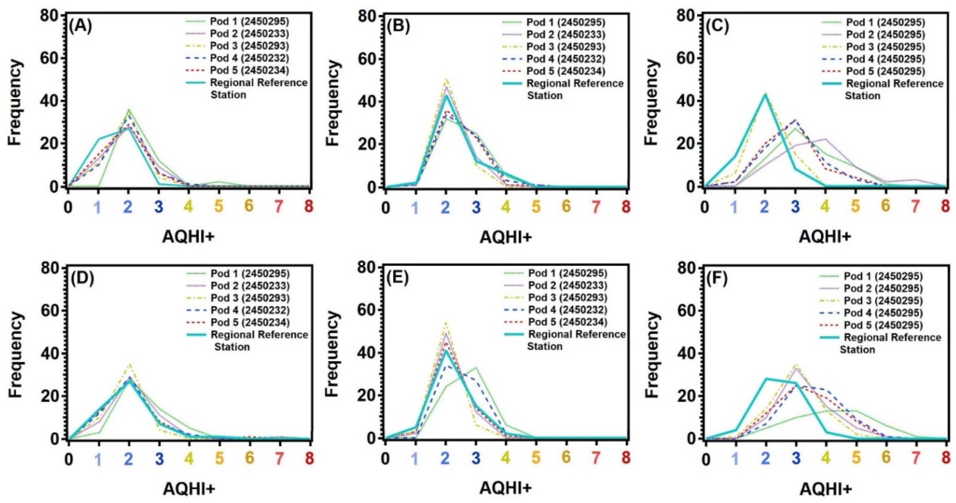
To assess the variations of AQHI+ across the pod network and in relation to the reference station, histograms were generated for each time period studied for both drop off and pickup times. These histograms compared the frequency of AQHI+ values recorded at each sensor pod in the AQMesh network in addition to comparisons with the reference station. These results, shown in Figure 3, illustrate that the multisensor network detects different levels of pollutants at each location, which can be attributed to the different emission sources near each pod location.
In addition, the impacts of seasonal variations on air quality are also observable in these figures. Figure 3A–C highlight the drop off time comparisons for fall, winter, and summer seasons, respectively. The peak frequency for the reference station is located at the AQHI+ value of 2 for all time periods, while the pod network is observed to have a lower frequency at this value caused by a higher frequency of AQHI+ values exceeding 2. This is most apparent in Figure 3C, where there are distinguishable peaks in the frequency of AQHI+ values ranging from 3 to 7. The analysis for the pickup times in Figure 3D–F highlights the increase in the AQHI+ value across all sites during pickup times. This observation is most apparent in Figure 3F, where the peak frequency for each sensor pod is larger than the value reported by the MECP. Pod 1, located near a highway, including access routes to the highway, has a peak at an AQHI+ value of 5, which is higher than the value reported by the MECP. Neighborhood scale variations in pollution are well known to be found in larger metropolitan cities [30]. The results in Figure 3 highlight that these variations can be found in smaller, less polluted cities, which is further supported by the findings of other research groups [31,32,33]. This variability in ambient contaminants was more precisely studied by Richards et al. [34], where a mobile mass spectrometer was used to map out the volatile organic compound sources across eastern Vancouver Island. These findings underline the inability of a single reference station to detect local hotspot regions in Kitchener, much less across the Region of Waterloo, and exemplifies the benefits of monitoring air quality using a multisensor network.
To further assess the AQHI+ values calculated for each pod in the network against the reference station, percentage mismatch comparisons were made for each period. This simple mismatch calculation per Equation (2) calculates the percentage of individual AQHI+ data points that exceed the reported values by the MECP for the same point in time for both drop off and pickup intervals by a index value of 1 or greater:
Figure 4A shows the percentage mismatch comparisons for the drop off time interval. This figure highlights the difference in pollutant emissions at each pod location. Pod 1, located near the highway, shows the largest mismatch values for all three seasons studied. This finding further supports the previous conclusion that the AQHI+ values are strongly influenced by traffic counts and local emission sources. Furthermore, this finding indicates that the current provincial monitoring station is not sufficient in accurately detecting AQHI+ fluctuations at the neighborhood scale, highlighting the need for pod networks to identify pollutant hotspots and the cause of these hotspots. When comparing the seasonal mismatch percentages in Figure 4A, it becomes apparent that the mismatch is also impacted by seasonal variations as mentioned in the long-distance scaling Section 3.3. With the formation of secondary pollutants being dependent on the availability of light to photochemically dissociate NO2, the AQHI+ values are also dependent on the availability of light [22,35]. Percentage mismatch values during the winter periods in Figure 4 are lower than the three seasons studied as they might have been influenced by the lockdown restrictions put in place between 23 December 2020 to 26 January 2021. Lingering restrictions over the following six weeks as shown in reference [36] and Supplementary Table S1 might also have contributed to this trend. This lockdown severely impacted the daily traffic counts which have reduced emissions during this period [23,37].
3.3. Analysis of Pod Network Outlier Points Using the Long-Distance Scaling Tool
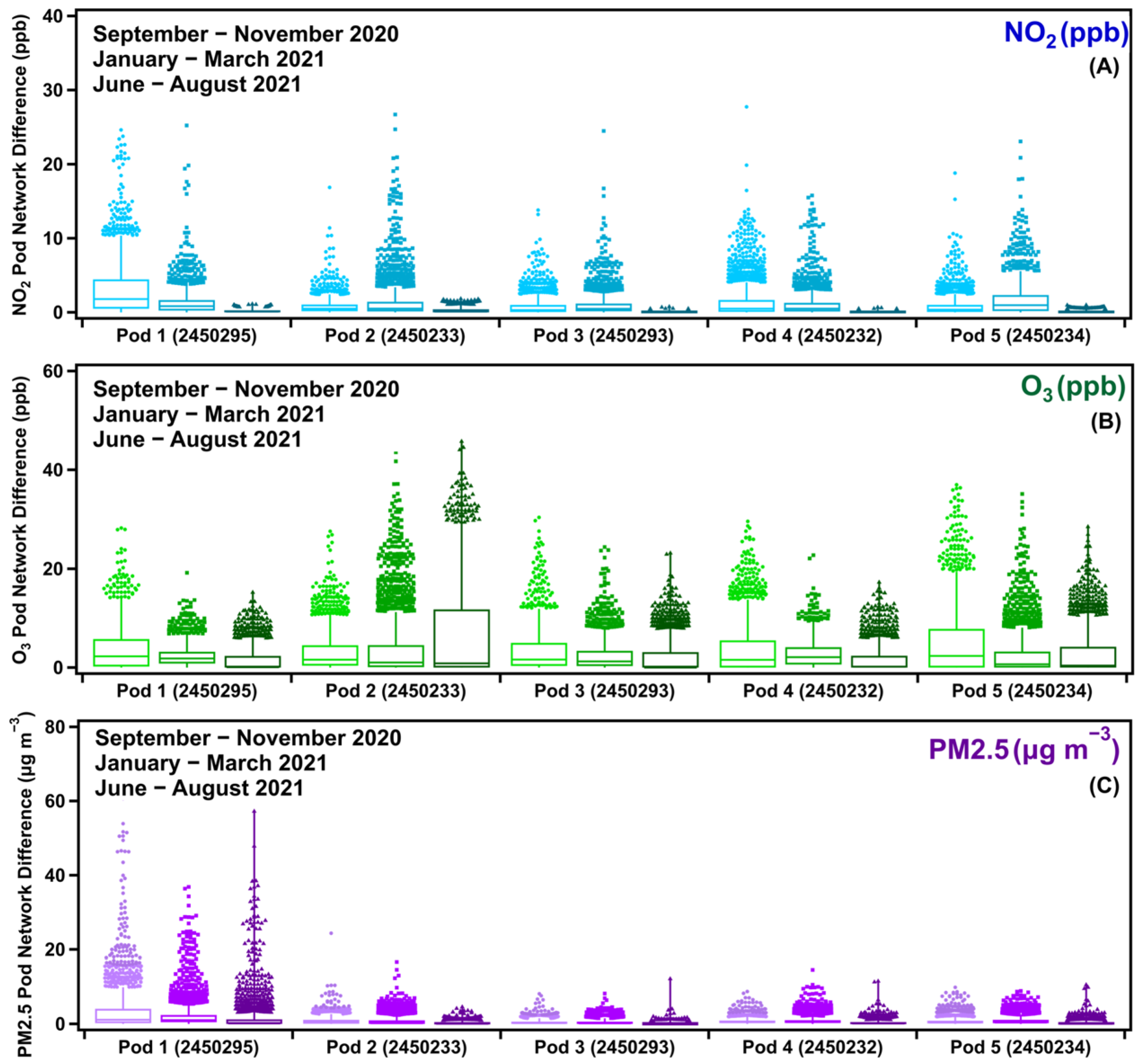
The long-distance scaling tool was designed to subtract the regional background of the pod network from each sensor pod to yield a pod network difference data set. One benefit of using this tool is that it scales the background of the AQMesh network to the background of the reference station in order to account for the weaker performance of the lower quality sensors in the AQMesh multisensor pods. If the sensors are measuring the same values as each other with no influence from local emission sources nearby, the difference would be zero (see Supplementary material on pod performance). The data presented in Figure 5 highlights the pod network data sets for the fall, winter, and summer seasons for NO2, O3, and PM2.5. A two-tailed t-test was used to compare the mean of each pod to the co-located pod (Pod 5), where the null hypothesis was that both mean values were equal. The results in Table S3 show that nearly all sensor pods in the network had statistically larger values for NO2 and PM2.5 as shown in Figure 5 A,C, respectively, illustrating the variations in pollutant levels at a hyperlocal scale. In addition, another two-tailed t-test was done using Pod 1 (near the highway) in place of the co-located pod, which showed that Pod 1 has statistically significant variations when compared to Pods 2–5 in the network (See Supplemental Tables S3 and S4). These findings suggest that highway traffic may influence detected pollutant levels to some extent. These findings further highlight how air quality metrics could vary from site to site (see Section 3.2).
A survey of the literature indicated that the PM2.5 levels downwind from factories would result in elevated PM2.5 levels [38]. Pod 4 is located downwind from a rubber factory and is in close proximity to King Street. Our initial hypothesis was that the September–November 2020 period would have the largest number of outlier points. However, our analysis did not show a clear influence of these emission sources on the observed concentrations of PM2.5 for pod 4 (squares shown in Figure 5C), which warrants further investigation. Seasonal variability was also found to play a role in the level of detected pollutants in the multisensor pod network. This seasonal effect is most evident in Figure 5A, where NO2 levels are highest when daylight hours are shorter (September–November; January–March), and lowest when daylight hours are long (January–August) (see reference [23] for solar irradiance data and correlation with NO2 levels). With NO2 being a secondary pollutant formed from the oxidation of nitric oxide (NO) [39], it became apparent that the comparison between different seasons is directly linked to the amount of light present that photolyzes NO2 [40].
The photochemically dissociated NO2 produces NO and oxygen atoms (O) as products. These oxygen atoms react with atmospheric oxygen in the presence of a chaperone molecule to form ground–level ozone. Thus, the formation of ground–level ozone is dependent on the level of photochemically dissociated NO2 [39,40], indicating that a anti–correlation exists between the two pollutants [37]. This anti–correlation was evident when comparing results for Pod 2 in Figure 5A,B, which show that NO2 levels declined in June–August 2021 while ground–level ozone values rose. Elevated NO2 has also been linked to traffic emissions as shown in the publication by Voordeckers et al. [36], which highlighted the statistically significant correlation between traffic counts and NO2. However, this observation is not clearly evident for all whisker plots shown in Figure 5, specifically for the January–March 2021 period.
3.4. Assessment of Carbon Monoxide (CO) Levels
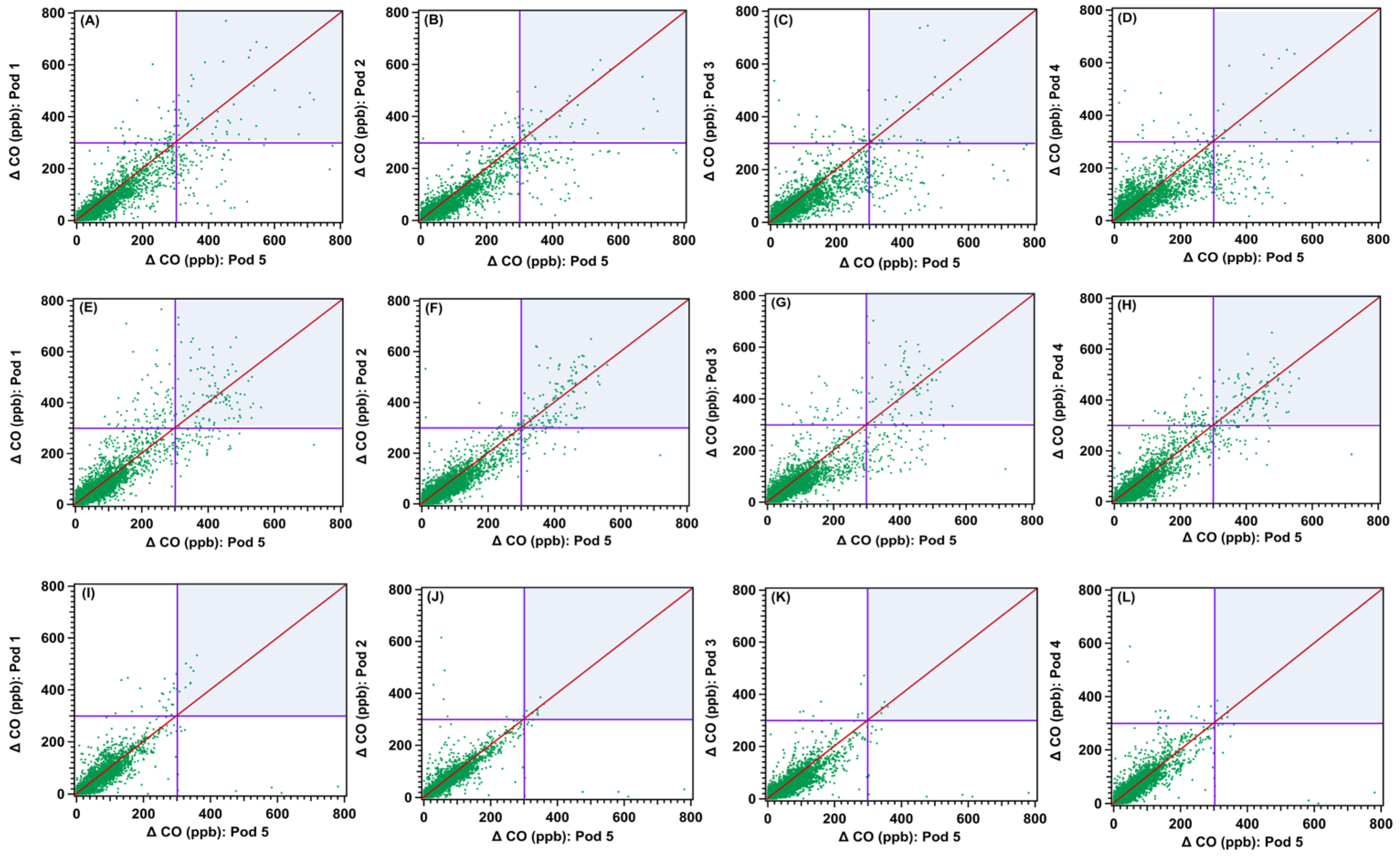
Carbon Monoxide is a colorless, odorless, and tasteless chemical. In large doses, this pollutant can have adverse effects on human health. Inhalation of this gas results in direct diffusion to the bloodstream, drastically inhibiting the oxygen transport pathways in the human body, causing organ failure. This is particularly dangerous for those who have underlying conditions such as heart disease, where the tolerance of this contaminant is significantly lower [29]. The reference station monitors NO, NO2, O3, and PM2.5 levels. However, the levels of CO emitted from the incomplete combustion of fuels used by vehicles are not monitored. These CO levels are known to interact with free hydroxyl radicals in the atmosphere, oxidizing CO to the well–known greenhouse gas, CO2 [5,39,40]. The AQMesh multisensor pods are capable of monitoring both CO and CO2 levels in the atmosphere through the electrochemical and NDIR sensors, respectively. In this section, we calculate the enhancement in CO and CO2 levels at each pod location and correlated with the co-located pod. The hypothesis is that pods located closer to traffic would experience relatively higher enhancement of CO levels above the regional background level compared to the co-located pod in a city park. The enhancement was calculated by taking the long-distance scaled dataset for each sensor pod and subtracting the background concentration as shown in Equation (3):
ΔCO (ppb) for Pod # = LDS Data (Pod #) − Background Concentration (Pod #)
In this study, the background CO was defined as the 10th percentile of the measured gas over a 24-h running window centered on each measurement (using data from the 12 h preceding and the 12 h following each measurement). Since the sensor pods collected data at a 15-min resolution, the running window consisted of 96 measurements (four measurements per hour by 24 h). This 10th percentile running window was calculated using an algorithm created in RStudio by Yuan You [41] (see Supplementary document for sample code). This analysis highlighted the ability of this sensor pod network to capture CO enhancement events as shown by the data points in the top right quadrant of Figure 6. The LOC for the detection of CO by the electrochemical sensor is <300 ppb>, which is shown as purple lines in the scatter plots. The CO sensor LOC is fairly close to the background concentration calculated for each pod in the network.
The datapoints found in the top right quadrant for each scatter plot in Figure 6 highlight the detectable local enhancements of CO levels for that particular site. Figure 6E–H show that CO levels enhanced during Winter 2021 and to a much smaller extent during Fall 2020 (Figure 6A–D). For summer 2021, the data in Figure 6I–L show that there is no detectable CO enhancement. The origin of these enhancements remains uncertain. One of the main conclusions from this analysis is that the lack of continuous traffic monitoring in Kitchener makes it difficult to correlate CO emissions to traffic. Preliminary analyses suggest that the origin of the photochemically active CO, which is short-lived in the atmosphere, arise from a combination of seasonal influences (sunlight exposure) and local emission sources. Additional studies need to be conducted prior to making any final conclusions. With CO being a pollutant of interest due to its health impacts, and the fact that these CO levels are elevated during events such as the wildfires, it is crucial to monitor this pollutant as further development in the region continues.
3.5. Case Study: Effects of Northern Ontario Wildfires on Local Air Quality
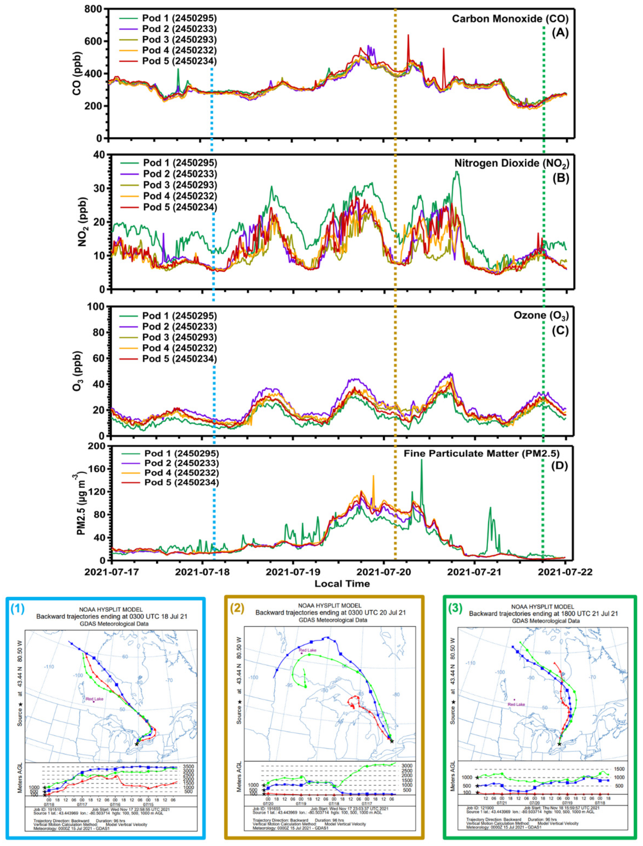
In summer 2021, several large forest fires were reported in the Red Lake area in Northwestern Ontario close to the Manitoba border. By 22 July 2021, two large fires were burning (51,000 hectares and 23,000 hectares) in the Red Lake area, as reported by CBC News [42]. In the weeks following the start of these fires, poor air quality and reduced visibility warnings were issued across Southern Ontario, located more than 1000 km from the wildfire smoke from Northwestern Ontario [43,44,45]. Based on data provided by the Ontario Ministry of Natural Resources and Forestry (see Table 3), there were a number of large fires burning in Red Lake in mid-July that appeared to impact pollutant levels in Kitchener.
Figure 7 shows the pollutant concentrations detected at each sensor pod for a series of pollutants. To observe the back trajectories for each pollutant, specific times were selected -as indicated in the vertical dashed lines- before (1), during (2), and after (3) the wildfire event, as denoted by the colored lines overlayed on the time series plots. The first back trajectory (1) shows air travelling from Northwestern Ontario to the north of Red Lake. The second back trajectory (2) shows that the air at the peak of the elevated levels came from within the vicinity of the Red Lake area. As this higher altitude smoke descended to lower levels within the boundary layer, and higher pollutant concentrations were detected by the multisensors in Kitchener. The third back trajectory (3) shows the air shifting to a northerly origin where there were far fewer fires burning during this time.
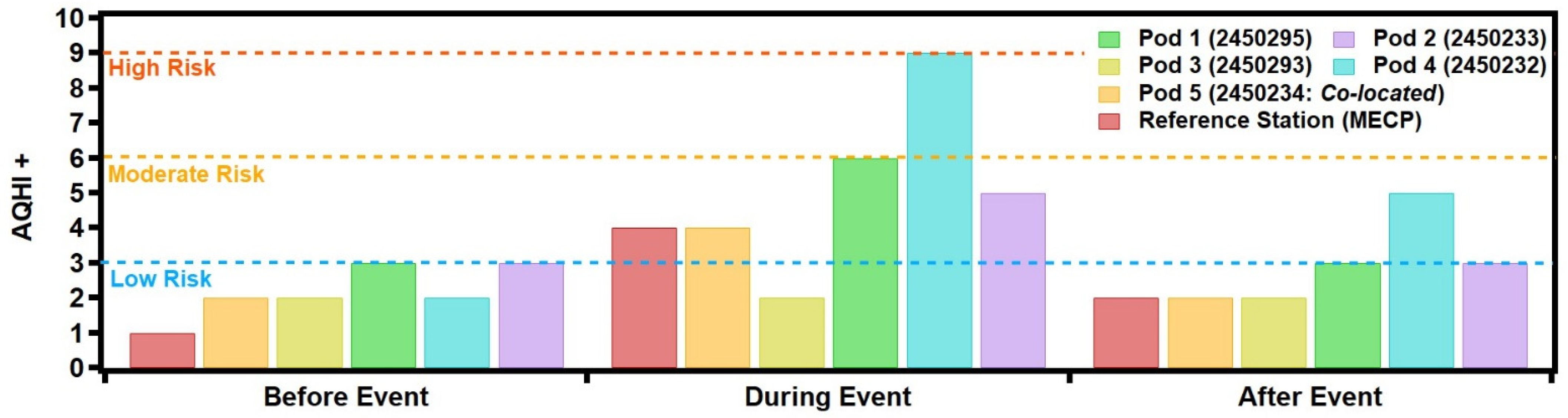
In addition to this back trajectory analysis, local AQHI+ values were calculated for all five pods in the multisensor network for comparison with those calculated using the reference station data. Figure 8 shows the results of these calculation for the three periods highlighted in Figure 7. Each event was captured very well from the network pod sensors, which detected higher levels of AQHI+ values for all time intervals studied, tracking with the increase and decrease seen at the reference station.
The interval during the event detected elevated concentrations of pollutants in Kitchener, likely to be caused by the large influx of particulate matter into the city. In addition, some sensor pods in the multisensor network detected pollutant levels far larger than what the MECP reported, particularly for Pods 2 and 4, which pushed the AQHI+ value into the high risk and moderate risk classifications of air quality, respectively, versus the low to moderate risk reported by the MECP. This observation was also shown, to a lesser extent, in the data for Pod 1. This analysis further highlights the potential impact of local sources to add to, and exacerbate, regional effects. Following the wildfire event, AQHI+ values dropped to lower levels again. However, some of the transported particulates are believed to have remained in the atmosphere during this time interval as shown by Pod 4 with a relatively higher AQHI+ value.
4. Conclusions
The use of multisensor mini air quality monitoring stations is rapidly increasing due to their ease of use and relatively low cost. The findings of this pilot study highlight the benefits of installing local AQMesh multisensor pod networks in suburban communities and shows that these pods work well in environments with lower pollution levels than large metropolitan cities. Measurements were made during a wide range of conditions, including clean air quality periods (pandemic lockdown) to polluted conditions (for example, wildfire smoke detection). The small sensor systems used in this project (AQMesh) illustrated relatively high correlation to the reference station for most pollutants of interest, despite not being co-located. NO2 showed a lower correlation over longer distances, but due to the more transient nature of NO2, this finding is expected. However, when using the long-distance scaling tool, all sensor species showed a high correlation to the reference, providing confidence in the scaling to be applied. The following conclusions were made based on our findings:
- The current provincial air quality monitoring infrastructure is not sufficient in accurately assessing pollutant levels at a neighbourhood scale in Kitchener. A network of multisensor pods is a viable alternative, which requires a mobile air quality station equipped with research grade equipment to regularly verify the pods’ performance,
- The multisensor pods used in this project are reasonably accurate in the detection of local pollutants relative to the reference station, particularly O3 and PM2.5,
- Pod 1, located near a regional highway, including access routes to the highway, has the largest concentration of NO2 and PM2.5 with higher frequencies of AQHI+ exceeding those reported by MECP for both dropoff (7–10 a.m.) and pickup (3–6 p.m.) school times, suggesting that traffic may play a significant role in local air quality,
- Preliminary analysis of CO emissions, which are not detected by the reference station, highlight the ability of the multisensor pods network to detect local CO enhancements caused by local emission sources and seasonal variations. Additional studies are needed to better assess the main contributor to these enhancement events,
- Wildfire events in Northwestern Ontario were captured by the pod network at a high data resolution of 15 min. Comparing the AQHI+ values at each period in the event highlights the potential impact of local sources to add to, and exacerbate, regional effects.
Supplementary Materials
The following supporting information can be downloaded at: https://www.mdpi.com/article/10.3390/atmos13010083/s1, Table S1: Provincial-led public health orders to limit the spread of COVID-19 in 2020–2021 in the province of Ontario (ON), Measuring the quality of AQMesh multisensor system performance, Table S2. Sensors used to collect pollutant data for the low-cost sensor pods (AQMesh)., Figure S1. Flowchart detailing the QA/QC and AQHI+ calculation protocol, Figure S2. Histograms generated for October 2020, Tables S3 and S4. Results for p-value calculations, and Sample R Statistics coding used to calculate the background concentration of CO for each pod in the sensor pod network.
Author Contributions
Conceptualization T.T. and H.A.A.-A.; Data curation, N.S.; Formal analysis, W.M., L.N. and A.A.; Funding acquisition, H.A.A.-A.; Investigation, N.S., L.N. and T.T.; Methodology, T.T., A.A. and H.A.A.-A.; Project administration, H.A.A.-A.; Resources, H.A.A.-A.; Software, T.T. and A.A.; Supervision, H.A.A.-A.; Validation, L.N., T.T. and A.A.; Visualization, W.M., N.S., L.N., T.T., A.A. and H.A.A.-A.; Writing—Original draft, W.M.; Writing—Review & editing, W.M., N.S., L.N., T.T., A.A. and H.A.A.-A. All authors have read and agreed to the published version of the manuscript.
Funding
The authors acknowledge funding from the City of Kitchener, NSERC Alliance Program for COVID-19 related research, and the Canadian Foundation for Innovation Exceptional Opportunities Fund. W.M. acknowledge the William Nikolaus Martin Entrance Scholarship for Graduate Students and the MS2 Discovery Institute Student Researcher Award.
Institutional Review Board Statement
Not applicable.
Informed Consent Statement
Not applicable.
Data Availability Statement
The data presented in this study are available on request from the corresponding author. The scaled data are publicly available on the Kitchener Air Quality Dashboard: https://Kitchenergis.maps.arcgis.com/apps/das-boards/fddc1fd0c5e84b459d7c04f5e4db1a7c (accessed on 20 September 2021).
Acknowledgments
All figures and tables were created by the authors. The authors gratefully acknowledge the NOAA Air Resources Laboratory (ARL) for the pro-vision of the HYSPLIT transport and dispersion model and/or READY website (https://www.ready.noaa.gov) (accessed on 20 September 2021) used in this publication.
Conflicts of Interest
T.T. works at AQmesh. The rest of the authors declare no conflict of interest.
References
- World Health Organization. Air Pollution. Available online: https://www.who.int/health-topics/air-pollution#tab=tab_1 (accessed on 8 June 2021).
- UNICEF. Pollution: 300 Million Children Breathing Toxic Air—UNICEF Report. Available online: https://www.unicef.org/press-releases/pollution-300-million-children-breathing-toxic-air-unicef-report (accessed on 2 November 2021).
- US EPA. Nitrogen Dioxide (NO2) Pollution. Available online: https://www.epa.gov/no2-pollution/basic-information-about-no2 (accessed on 21 June 2021).
- Gentner, D.R.; Jathar, S.H.; Gordon, T.D.; Bahreini, R.; Day, D.A.; El Haddad, I.; Hayes, P.L.; Pieber, S.M.; Platt, S.M.; de Gouw, J.; et al. Review of Urban Secondary Organic Aerosol Formation from Gasoline and Diesel Motor Vehicle. Environ. Sci. Technol. 2017, 51, 1074–1093. [Google Scholar] [CrossRef]
- Sillman, S. Overview: Tropospheric Ozone, Smog and Ozone-NOx-VOC Sensitivity. Available online: http://www-personal.umich.edu/~sillman/ozone.htm (accessed on 16 November 2021).
- Kroll, J.H.; Seinfield, J.H. Chemistry of secondary organic aerosol: Formation and evolution of low volatility organics in the atmosphere. Atmos. Environ. 2008, 42, 3593–3624. [Google Scholar] [CrossRef]
- Carlson, A.; Burtraw, D. Lessons from the Clean Air Act: Building Durability and Adaptability into US Climate and Energy Policy; Cambridge University Press: Cambridge, UK, 2019. [Google Scholar]
- Grennfelt, P.; Engleryd, A.; Forsius, M.; Hov, Ø.; Rodhe, H.; Cowling, E. Acid rain and air pollution: 50 years of progress in environmental science and policy. Amibo 2019, 49, 849–864. [Google Scholar] [CrossRef]
- Human Toxicology and Air Standards Section; Technical Assessment and Standards Development Branch; Ontario Ministry of the Environment (MECP). Ambient Air Quality Criteria. MECP, Toronto, ON, Canada. 2020. Available online: https://www.ontario.ca/page/ontarios-ambient-air-quality-criteria#section-4 (accessed on 28 January 2021).
- BreatheLife. What Are the W.H.O Air Quality Guidelines? Available online: https://breathelife2030.org/news/w-h-o-air-quality-guidelines/ (accessed on 16 October 2021).
- Region of Waterloo Demographics. Available online: https://www.regionofwaterloo.ca/en/doing-business/demographics.aspx (accessed on 21 January 2021).
- Climate Action Plans. Available online: https://climateactionwr.ca/climate-action-plans/#long-term (accessed on 17 March 2021).
- Environmetnal Defense Fund (EDF). Breathe London Blueprint. Available online: https://www.globalcleanair.org/blueprint/ (accessed on 21 November 2021).
- Borée Project: Experimenting with a Ventilation Optimization Device to Preserve the Local Populations at the Head of the L2 Tunnel. Available online: https://www.atmosud.org/actualite/projet-boree-experimenter-un-dispositif-doptimisation-de-la-ventilation-pour-preserver-les (accessed on 12 October 2021).
- Vadali, M. Assessing Urban Air Quality project. Available online: https://www.pca.state.mn.us/air/assessing-urban-air-quality-project (accessed on 27 October 2021).
- AQMesh. About AQMesh: Product timeline. Available online: https://www.aqmesh.com/about/ (accessed on 26 November 2021).
- AQMesh. Operating Manual. Available online: https://www.aqmesh.com/media/lw4i2qzy/aqmesh-operating-manual.pdf (accessed on 10 September 2021).
- Duvall, R.; Clements, A.; Hagler, G.; Kamal, A.; Goodman, L.; Frederick, S.; Barkjohn, K.; von Wald, I.; Greene, D.; Dye, T. Performance Testing Protocols, Metrics, and Target Values for Ozone Air Sensors: Use in Ambient, Outdoor, Fixed Site, Non-Regulatory and Informational Monitoring Applications; EPA/600/R-20/279; U.S. Environmental Protection Agency, Office of Research and Development: Washington, DC, USA, 2021.
- Dhall, S.; Mehta, B.R.; Tyage, A.K.; Sood, K. A review on environmental gas sensors: Materials and technology. Sens. Int. 2021, 2, 1–10. [Google Scholar] [CrossRef]
- Zhu, Y.; Shi, J.; Zhang, Z.; Zhang, C.; Zhang, X. Development of a gas sensor utilizing chemiluminescence on nanosized titanium dioxide. Anal. Chem. 2002, 74, 120–124. [Google Scholar] [CrossRef]
- Munir, S.; Mayfield, M.; Coca, D.; Jubb, S.A.; Osammor, O. Analysing the performance of low-cost air quality sensors, their drivers, relative benefites and calibration in cities—A case study in Sheffield. Environ. Monit. Assess. 2019, 191, 1–22. [Google Scholar] [CrossRef]
- Pöschl, U.; Shiraiwa, M. Multiphase Chemistry at the Atmosphere−Biosphere Interface Influencing Climate and Public Health in the Anthropocene. Chem. Rev. 2015, 115, 4440–4475. [Google Scholar] [CrossRef] [PubMed]
- Al-Abadleh, H.A.; Lysy, M.; Neil, L.; Patel, P.; Mohammed, W.; Khalaf, Y. Rigorous quantification of statistical significance of the COVID-19 lockdown effect on air quality: The case from ground-based measurements in Ontario, Canada. J. Haz. Mater. 2021, 413, 1–17. [Google Scholar] [CrossRef]
- US EPA. Instruction Guide and Macro Analysis Tool: Evaluating Low-Cost Air Sensors by Collocation with Federal Reference Monitors. Available online: https://www.epa.gov/air-research/instruction-guide-and-macro-analysis-tool-evaluating-low-cost-air-sensors-collocation (accessed on 15 December 2021).
- Government of Canada. The Air Quality Health Index: How Air Pollution Affects Your Health Fact Sheet. 2015. Available online: https://www.canada.ca/content/dam/eccc/migration/main/cas-aqhi/47327a59-009d-4ca2-aedd-29698305d4a0/aqhi-factsheet-2015-en.pdf (accessed on 1 November 2021).
- Yao, J.; Steib, D.M.; Taylor, E.; Henderson, S.B. Assessment of the Air Quality Health Index (AQHI) and four alternate AQHI-plus amendments for wildfire seasons in British Colombia. Can. J. Public Health 2019, 111, 96–106. [Google Scholar] [CrossRef] [PubMed]
- Chen, H.; Copes, R. Review of Air Quality Index and Air Quality Health Index; Public Health Ontario: Toronto, ON, Canada, 2013. [Google Scholar]
- Steib, D.M.; Burnett, R.T.; Doiron, M.S.; Brion, O.; Shin, H.H.; Economou, V. A New Multipollutant, No-Threshold Air QualityHealth Index Based on Short-Term Associations Observed in Daily Time-Series Analyses. J. Air Waste Manag. Assoc. 2008, 58, 435–450. [Google Scholar] [CrossRef] [PubMed]
- Ministry of the Environment. Air Quality in Ontario 2014 Report; 2014; p. 34. Available online: http://www.airqualityontario.com/downloads/AirQualityInOntarioReportAndAppendix2014.pdf (accessed on 14 December 2021).
- Gaoa, Y.; Wangb, Z.; Liud, C.; Pengc, Z. Assessing neighborhood air pollution exposure and its relationship with the urban form. Build. Environ. 2019, 155, 15–24. [Google Scholar] [CrossRef]
- Mohtar, A.A.A.; Latif, M.T.; Bahrudin, N.H.; Ahamad, F.; Chung, J.X.; Othman, M.; Juneng, L. Variation of major air pollutants in different seasonal conditions in an urban environmen in Malaysia. Geosci. Lett. 2018, 5, 1–13. [Google Scholar] [CrossRef]
- Markandeya; Verma, P.K.; Mishra, V.; Singh, N.K.; Shukla, S.P.; Mohan, D. Spatio-temporal assessment of ambient air quality, their health effects, and improvement during COVID-19 locdown in one of the most polluted cities in India. Environ. Sci. Pollut. Res. 2020, 28, 10536–10551. [Google Scholar] [CrossRef]
- Tabinda, A.B.; Habib, Q.; Yasar, A.; Rasheed, R.; Mahmood, A.; Iqbal, A. Ambient Air Quality of Faisalabad with Relevance to the Seasonal Variations. MAPAN-J. Metrol. Soc. India 2020, 35, 421–426. [Google Scholar] [CrossRef]
- Richards, L.C.; Davey, N.G.; Gill, C.G.; Krogh, E.T. Discrimination and geo-spatial mapping of atmospheric volatile organic compound sources using full scan direct mass spectral data collected from a moving vehicle. Environ. Sci. Process. Impacts 2020, 22, 173–186. [Google Scholar] [CrossRef]
- Benton, A.K.; Langridge, J.M.; Ball, S.M.; Bloss, W.J.; Dall’Osto, M.; Nemitz, E.; Harrison, R.M.; Jones, R.L. Night-time chemistry above London: Measurements of NO3 and N2O5 from the BT Tower. Atmos. Chem. Phys. 2010, 10, 9781–9795. [Google Scholar] [CrossRef]
- Voordeckers, D.; Meysman, F.J.R.; Billen, P.; Tytgat, T.; Van Acker, M. The impact of street canyon morphology and traffic volume on NO2 values in the street canyons of Antwerp. Build. Environ. 2021, 197, 1–10. [Google Scholar] [CrossRef]
- Hashim, B.M.; Al-Naseri, S.K.; Al-Maliki, A.; Al-Ansari, N. Impact of COVID-19 lockdown on NO2, O3, PM 2.5 and PM10 concentrations and assessing air quality changes in Baghdad, Iraq. Sci. Total Environ. 2021, 754, 1–10. [Google Scholar] [CrossRef]
- Rattanavaraha, W.; Chu, K.; Budisulistiorini, S.H.; Riva, M.; Lin, Y.H.; Edgerton, E.S.; Baumann, K.; Shaw, S.L.; Guo, H.; King, L.; et al. Assessing the impact of anthropogenic pollution on isoprene-derived secondary organic aerosol formation in PM2.5 collected from the Birmingham, Alabama, ground site during the 2013 Southern Oxidant and Aerosol Study. Atmos. Chem. Phys. 2016, 16, 4897–4914. [Google Scholar] [CrossRef]
- Atmospheric Chemistry at Night. Available online: https://www.rsc.org/images/environmental-brief-no-3-2014_tcm18-237724.pdf (accessed on 24 November 2021).
- Akimoto, H.; Hirokawa, J. Atmospheric Multiphase Chemistry: Fundamentals of Secondary Aerosol Formation; Wiley: Hoboken, NJ, USA, 2020; p. 544. [Google Scholar]
- You, Y.; Byrne, B.; Colebatch, O.; Mittermeier, R.L.; Vogel, F.; Strong, K. Quantifying the Impact of the COVID-19 Pandemic Restrictions on CO, CO2, and CH4 in Downtown Toronto Using Open-Path Fourier Transform Spectroscopy. Atmosphere 2021, 12, 848. [Google Scholar] [CrossRef]
- Air Quality Concerns Heighten Due to Smoke from 166 Forest Fires in Northwestern Ontario. CBC News, 22 July 2021. Available online: https://www.cbc.ca/news/canada/thunder-bay/forest-fire-air-quality-july-22-1.6112543(accessed on 16 November 2021).
- Thompson, C. Forest Fire Smoke Likely to Affect Air Quality all Week in Waterloo Region. The Record, 26 July 2021. Available online: https://www.therecord.com/news/waterloo-region/2021/07/26/forest-fire-smoke-likely-to-affect-air-quality-all-week.html?rf(accessed on 16 November 2021).
- Eppel, B. Wildfire Smoke Expected to Linger in Waterloo Region until Wednesday. City News, 19 July 2021. Available online: https://kitchener.citynews.ca/local-news/wildfire-smoke-expected-to-linger-in-waterloo-region-until-wednesday-3968245(accessed on 16 November 2021).
- Agnihotri, A. Forest Fires Reduce Air Quality across Southern Ontario. Toronto Star, 19 July 2021. Available online: https://www.thestar.com/news/gta/2021/07/19/forest-fires-reduce-air-quality-across-southern-ontario.html?rf(accessed on 16 November 2021).
- Forestry. Forest Fire Info Map. Available online: https://www.lioapplications.lrc.gov.on.ca/ForestFireInformationMap/index.html?viewer=FFIM.FFIM (accessed on 15 November 2021).
- Stein, A.F.; Draxler, R.R.; Rolph, G.D.; Stunder, B.J.B.; Cohen, M.D.; Ngan, F. NOAA’s HYSPLIT atmospheric transport and dispersion modeling system. Am. Met. Soc. 2015, 96, 2059–2077. [Google Scholar] [CrossRef]
- Rolph, G.; Stein, A.; Stunder, B. Real-time Environmental Applications and Display System: READY. Environ. Model. Softw. 2017, 95, 210–228. [Google Scholar] [CrossRef]
Figure 1.
Spatial location of multisensor pods in Kitchener, ON. Pod 2450233 and Pod 2450293 are located near major roads. Pod 2450232 was located downwind from a factory (western location, September 2020 to December 2020), and was moved to near a main road (eastern location, December 2020–present). Pod 2450295 is located near Highway 8, and the co-located pod (Pod 2450234) is located within 30 m of the reference station used by the MECP. See Table 2 for additional details on the coordinates and associated location.

Figure 2.
Regression plots of NO2, O3 and PM2.5 comparing the co-located AQMesh pod (2450234, y-axis) with the MECP reference station (x-axis) for 22 September–22 November 2020 (A–C), 4 January–31 March 2021 (D–F), and 1 June–31 August 2021 (G–I). The WHO AQG (2021) are shown as dashed green lines in each regression plot. The solid red line is the regression line of best fit with R2 values on the bottom right corner. The red diamond markers denote the LOC for each pollutant as shown in the Supplementary Section.

Figure 3.
Histograms comparing the AQHI+ value frequency for each pod in the multisensor network in addition to the MECP reference station for drop off time intervals in (A) Fall 2020, (B) Winter 2021, and (C) Summer 2021, and for pickup time intervals in (D) Fall 2020, (E) Winter 2021, and (F) Summer 2021.

Figure 4.
Percentage mismatch values calculated for all pods in the low-cost network for each time period. (A) Dropoff time interval comparisons across all network pods, (B) Pickup time intervals across all pod networks.
Figure 4.
Percentage mismatch values calculated for all pods in the low-cost network for each time period. (A) Dropoff time interval comparisons across all network pods, (B) Pickup time intervals across all pod networks.

Figure 5.
Pod network difference values obtained from the custom-made long distance scaling tool to highlight the outlier data points observed for each pod throughout the Fall 2020, Winter 2021, and Summer 2021 time periods. Results were plotted for (A) Nitrogen Dioxide (NO2), (B) Ground-level Ozone (O3), and (C) Fine Particulate Matter (PM2.5). Note Pod 4 September–November 2020 was in a different location than the other two periods.

Figure 6.
Scatter plots comparing the CO levels of the co-located pod against other pods in the network. (A–D) illustrate the scatter plots for the Fall 2020 time period, (E–H) illustrates the scatter plots for the Winter 2021 period, and (I–L) illustrates the scatter plots for the Summer 2021 period. The top right quadrant highlighted in blue denotes the CO enhancement quadrant.

Figure 7.
Time series of pollutant levels detected at all sites during wildfire episode for (A) CO, (B) NO2, (C) O3, and (D) PM2.5. Data presented is for 17–21 July 2021, where air quality warnings were issued in Southern Ontario on 19 July and 20 July 2021. Lower panel figures (1–3) show the back trajectory analyses from the NOAA Air Resources Laboratory HYSPLIT transport and dispersion model, including 96 h back trajectories ending in Victoria, Kitchener (UTM 17T 540140 E, 4810258 N). Three heights were chosen (100 m, 500 m and 1000 m) to account for a range of heights above Kitchener. The three sets of analyses show the back trajectory ending (1) before the event on 17 July 2021 at 22:00 (EST), (2) during the event on 19 July 2021 at 22:00 (EST), and (3) after the event on 21 July 2021 at 13:00 (EST) [47,48].

Figure 8.
AQHI+ values captured by the sensor pods in the multisensor pod network in relation to the AQHI+ values captured at the reference station. Results illustrate significantly larger readings for Pod 4 during the event period.
Figure 8.
AQHI+ values captured by the sensor pods in the multisensor pod network in relation to the AQHI+ values captured at the reference station. Results illustrate significantly larger readings for Pod 4 during the event period.


Table 1.
Short-term outdoor exposure limits outlined in the most recently published Ontario AAQC [9] and the recently published 2021 WHO AQG Criteria [10].
| Gas | WHO AQG (2021) | Ontario AAQC Limits (2020) |
|---|---|---|
| NO2 | 13 ppb (24 h) | 100 ppb (24 h) |
| O3 | 50 ppb (8 h) | 80 ppb (1 h) |
| PM2.5 | 15 µg m−3 (24 h) | 28 µg m−3 (24 h) |
| SO2 | 15 ppb (24 h) | 40 ppb (1 h) |
Table 2.
Classification, UTM Coordinate location, and elementary school associated with each sensor pod in the low-cost sensor network.
Table 2.
Classification, UTM Coordinate location, and elementary school associated with each sensor pod in the low-cost sensor network.
| Pod Number | Pod ID | UTM Coordinates | Associated Location | ||
|---|---|---|---|---|---|
| Zone | Easting | Northing | |||
| Pod 1 | 2450295 | 17 T | 541107 | 4809056 | St. Bernadette (School) |
| Pod 2 | 2450233 | 17 T | 540152 | 4809823 | JF Carmichael (School) |
| Pod 3 | 2450293 | 17 T | 541824 | 4811246 | Suddaby (School) |
| Pod 4 | 2450232 | 17 T | 540000 | 4811398 | King Edward (School) 1 |
| 17 T | 543590 | 4811325 | Smithson (School) | ||
| Pod 5 | 2450234 | 17 T | 540140 | 4810258 | Victoria Park (City Park) 2 |
1 The data collected from Pod 3 (west side of the main road) showed high levels of pollutant emissions. To further validate that these observations were in fact real, Pod 4 was moved in December 2020 from near a rubber factory (King Edward) to the east side of this main road (Smithson) and remains at this second location to this day. 2 Co-located pod (Pod 5: ID 2450234) was located within a 30 m range of the regional reference station.
Table 3.
Sample of wildfire durations and range in Northwestern Ontario obtained from the Ontario Ministry of Natural Resources and Forestry open-access data [46].
Table 3.
Sample of wildfire durations and range in Northwestern Ontario obtained from the Ontario Ministry of Natural Resources and Forestry open-access data [46].
| Name | District | Total Extent (ha) | Date Started | Date Fire Was Officially out 1 |
|---|---|---|---|---|
| RED102 | Red Lake | 2909.5 | 14 July 2021 | 14 September 2021 |
| RED108 | Red Lake | 20,831.1 | 14 July 2021 | 14 September 2021 |
| RED111 | Red Lake | 1543.1 | 15 July 2021 | 14 September 2021 |
| RED114 | Red Lake | 35,646.6 | 15 July 2021 | 14 September 2021 |
| RED120 | Red Lake | 3627.9 | 16 July 2021 | 14 September 2021 |
| RED137 | Red Lake | 5779.8 | 18 July 2021 | 14 September 2021 |
1 Personal communication with Ministry of Northern Development, Mines, Natural Resources and Forestry.
Publisher’s Note: MDPI stays neutral with regard to jurisdictional claims in published maps and institutional affiliations. |
© 2022 by the authors. Licensee MDPI, Basel, Switzerland. This article is an open access article distributed under the terms and conditions of the Creative Commons Attribution (CC BY) license (https://creativecommons.org/licenses/by/4.0/).
Share and Cite
MDPI and ACS Style
Mohammed, W.; Shantz, N.; Neil, L.; Townend, T.; Adamescu, A.; Al-Abadleh, H.A. Air Quality Measurements in Kitchener, Ontario, Canada Using Multisensor Mini Monitoring Stations. Atmosphere 2022, 13, 83. https://doi.org/10.3390/atmos13010083
AMA Style
Mohammed W, Shantz N, Neil L, Townend T, Adamescu A, Al-Abadleh HA. Air Quality Measurements in Kitchener, Ontario, Canada Using Multisensor Mini Monitoring Stations. Atmosphere. 2022; 13(1):83. https://doi.org/10.3390/atmos13010083
Chicago/Turabian StyleMohammed, Wisam, Nicole Shantz, Lucas Neil, Tom Townend, Adrian Adamescu, and Hind A. Al-Abadleh. 2022. "Air Quality Measurements in Kitchener, Ontario, Canada Using Multisensor Mini Monitoring Stations" Atmosphere 13, no. 1: 83. https://doi.org/10.3390/atmos13010083
Note that from the first issue of 2016, this journal uses article numbers instead of page numbers. See further details here.