Amy Stidworthy - Optimising local air quality models with sensor data - DMUG17
Download as PPTX, PDF1 like1,340 views
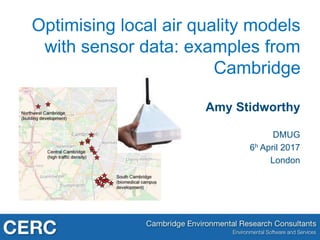
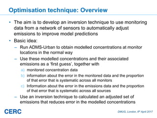
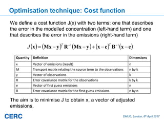
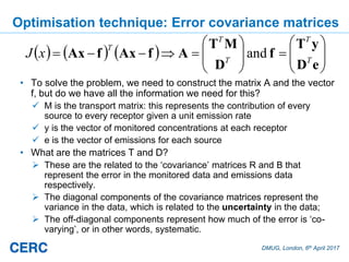
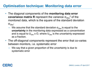
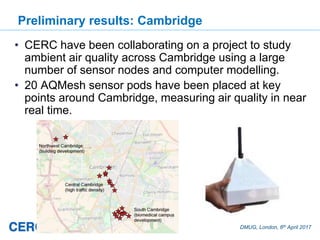
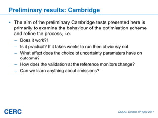
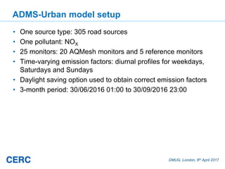
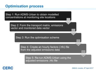
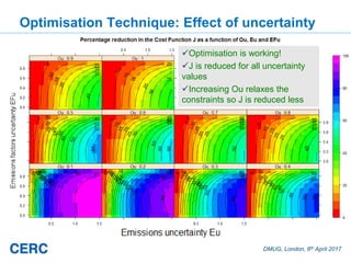
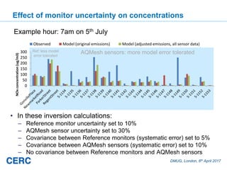
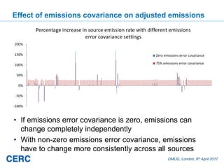
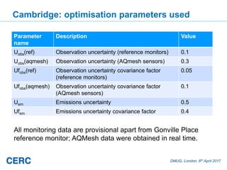
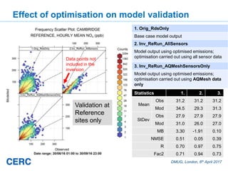
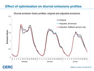
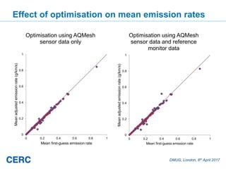
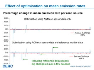
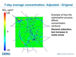
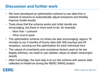
The document summarizes an optimization technique used to adjust air pollution emissions rates in an air quality model using data from low-cost air quality sensors. The technique develops an inversion method to automatically adjust emissions inputs to improve model predictions against monitored concentrations. Preliminary tests of the technique in Cambridge, UK optimized NOx emissions rates from 305 road sources against data from 20 low-cost sensors and 5 reference monitors. The optimization reduced errors between modeled and monitored concentrations and adjusted emissions profiles and rates in a physically reasonable manner.
1 of 30
Downloaded 69 times
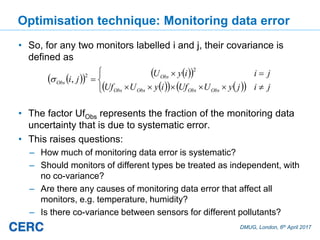
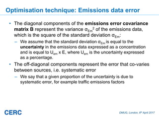
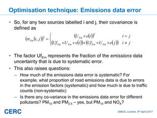
![DMUG, London, 6th April 2017
Optimisation technique: Introduction
• There are some conditions that have to be satisfied for such a
scheme to work:
a) The model concentration must be proportional to the emissions,
which means that complex effects like chemistry have to be
ignored
b) Any sources included must affect at least one receptor (monitor)
c) Any receptor included must have non-zero concentration
• The technique developed uses a probabilistic approach
following work by others, for example as used by the Met
Office for estimating volcanic ash source parameters using
satellite retrievals [Webster et al, 2016]](https://image.slidesharecdn.com/amystidworthy-optimisinglocalairqualitymodelswithsensordata-dmug17-170407093339/85/Amy-Stidworthy-Optimising-local-air-quality-models-with-sensor-data-DMUG17-6-320.jpg)

Recommended
Marc stettler modelling of instantaneous vehicle emissions - dmug17


Marc stettler modelling of instantaneous vehicle emissions - dmug17IES / IAQM DMUG remains the key annual event for experts in this field. Unmissable speakers will be examining topical issues in emissions, exposure and dispersion modelling.
Roger Barrowcliff - Chairman's introduction to vehicle section - DMUG17


Roger Barrowcliff - Chairman's introduction to vehicle section - DMUG17IES / IAQM An unapologetically technical conference, DMUG remains the key annual event for experts in this field. Unmissable speakers will be examining topical issues in emissions, exposure and dispersion modelling.
Dr James Tate - Better estimation of vehicle emissions for modelling - DMUG17


Dr James Tate - Better estimation of vehicle emissions for modelling - DMUG17IES / IAQM An unapologetically technical conference, DMUG remains the key annual event for experts in this field. Unmissable speakers will be examining topical issues in emissions, exposure and dispersion modelling.
Dr Glyn Rhys-Tyler - Road vehicle exhaust emissions; 'an age of uncertainty' ...


Dr Glyn Rhys-Tyler - Road vehicle exhaust emissions; 'an age of uncertainty' ...IES / IAQM DMUG remains the key annual event for experts in this field. Unmissable speakers will be examining topical issues in emissions, exposure and dispersion modelling.
Emma Gibbons - Model uncertainty in the assessment of major infrastructure pr...


Emma Gibbons - Model uncertainty in the assessment of major infrastructure pr...IES / IAQM DMUG remains the key annual event for experts in this field. Unmissable speakers will be examining topical issues in emissions, exposure and dispersion modelling.
Session 38 Xiaoliang Ma


Session 38 Xiaoliang MaTransportforum (VTI) This document summarizes research on integrating traffic and emission models to simulate the impacts of traffic on emissions. It describes:
1) Developing an approach to combine traffic simulation and emission models in a distributed way.
2) Proposing a method to calibrate microscopic emission models using aggregate emission measures.
3) Applying the integrated models to evaluate how different traffic demands and signal controls impact emissions.
Ermes-group presentation


Ermes-group presentationermes-group The ERMES Group coordinates research on mobile emission sources in Europe. It brings together transport emission modellers, researchers, funding agencies, and industry representatives. ERMES aims to become a permanent network that coordinates research programs to improve transport emission inventories in Europe. Key activities include harmonizing emission measurement procedures, sharing emission data, overseeing leading vehicle emission models like COPERT and HBEFA, and prioritizing future research issues.
Land gem v 3


Land gem v 3Umangi Mehta LandGEM is a Microsoft Excel-based tool that estimates landfill gas emissions, including methane and other pollutants, from municipal solid waste landfills. It uses a first-order decomposition rate equation to model emissions over time based on landfill-specific characteristics and waste acceptance rates entered by the user. The model consists of worksheets for inputs, outputs, graphs, and a report. It provides a simple approach to estimate emissions but has limitations such as not accounting for changes in landfill operations.
IRJET- Study of Vehicular Exhaust Emission Estimation


IRJET- Study of Vehicular Exhaust Emission EstimationIRJET Journal This study examined vehicular exhaust emissions using experimental testing and the COPERT emissions model. Researchers measured carbon monoxide (CO), hydrocarbon (HC), and nitrogen oxide (NOx) emissions from vehicle exhaust under different operating conditions, including idling and driving cycles. Emissions were compared to COPERT estimates. While CO and HC emissions correlated well with COPERT, measured NOx levels were higher. The study found CO emissions were overestimated by COPERT, while NOx was underestimated. Critical vehicle speeds that impact CO and NOx variations were identified. The research provides insight into exhaust emissions and helps validate the COPERT model.
LandGEM


LandGEMAnusha Srinivasan This is a presentation giving an introduction to the LandGEM model released by USEPA. It takes the student through a quick case study of the Pirana Landfill in India.
Meant for educational purposes only.
Improved Emissions Inventories for NOx and Particulate Matter from Small Comb...


Improved Emissions Inventories for NOx and Particulate Matter from Small Comb...Environmental Protection Agency, Ireland This document summarizes two projects aimed at improving emissions inventories for Ireland. The first project aims to develop accurate emission factors for NOx and particulate matter from small combustion installations like residential heating. Researchers are taking real-world measurements using testing equipment on a combustion rig with an Irish duty cycle. The second project aims to estimate road vehicle emissions using methods like ARTEMIS, which models emissions based on driving cycles and vehicle parameters. Researchers are collecting real-world driving data using onboard diagnostics loggers to input into emissions models.
Duncan Laxen - DMUG 2014


Duncan Laxen - DMUG 2014IES / IAQM At the 2014 annual Dispersion Modellers user group meeting guest speaker Duncan Laxen spoke on the topic: 'Linking ADMS with micro-simulation models'
CAMS GA Emissions


CAMS GA EmissionsCopernicus ECMWF - The document discusses the need to update the anthropogenic and biogenic emissions datasets used in CAMS simulations and analyses.
- It describes work being done to develop new, higher resolution global and European anthropogenic emissions inventories based on recent developments and incorporating temporal and speciation information.
- Issues with current datasets like inconsistent species emissions and lack of recent years are noted. Developing updated datasets exceeds current contract scopes.
- Evaluation of inverse modeling results and recommendations for improving emissions specification, resolution and temporal profiles are discussed.
Yvonne Brown - DMUG 2014


Yvonne Brown - DMUG 2014IES / IAQM At the 2014 annual Dispersion Modellers user group meeting guest speaker Yvonne Brown spoke on 'Changes to the Emission Factor Toolkit'
Towards a concept for the integration of European TCCON sites into the Resea...


Towards a concept for the integration of European TCCON sites into the Resea...Integrated Carbon Observation System (ICOS) The document discusses integrating European TCCON sites into the ICOS Research Infrastructure. TCCON provides complementary and reference data for satellite validation by measuring total column concentrations of greenhouse gases. Currently, European TCCON sites rely on short-term project funding, threatening continued operations. Integrating sites into ICOS could provide long-term funding and support from a proposed Atmospheric Column Thematic Centre. This would help preserve the network while centralizing quality control, data handling, and supporting innovation to improve satellite validation and calibration efforts. However, some open issues around instrumentation, data exchange, and national funding commitments would still need to be addressed.
Acme issec 


Acme issec Rajiv Ganguly This document presents a study applying a General Finite Line Source Model (GFLSM) to predict hydrocarbon concentrations on the M50 motorway in Ireland. The study compares monitored hydrocarbon data to concentrations modeled by GFLSM and the CALINE4 model at receptor points along the motorway. Results show that at distances of 25 meters and 120 meters from the road, GFLSM predictions matched monitored data better than CALINE4. At 240 meters, both models showed similar accuracy compared to monitored data. Overall, the study found GFLSM to be a satisfactory model for predicting vehicular air pollution along the M50 motorway.
Imperfect reversibility of air transport demand


Imperfect reversibility of air transport demandInstitute for Transport Studies (ITS) Presentation given by Dr Zia Wadud at the18th World Conference of the Air Transport Research Society, Bordeaux, France, July 2014.
atrs2014.org
www.its.leeds.ac.uk/people/z.wadud
Routes to Clean Air 2016 - Dr Norbert Ligterink - TNO


Routes to Clean Air 2016 - Dr Norbert Ligterink - TNOIES / IAQM Talk title: NOx and NO2 Emissions of diesel vehicles.
Routes to Clean Air is a two-day conference from the IAQM where academics, professionals and policy makers share their experiences of improving traffic emissions.
This event highlights the importance of public communication and behavioural change surrounding road transport and air quality issues.
Christine McHugh - DMUG 2014


Christine McHugh - DMUG 2014IES / IAQM At the 2014 annual Dispersion Modellers user group meeting guest speaker Christine McHugh spoke on the topic: 'Comparison of Air Quality in World Cities'
From copert2 to copert4


From copert2 to copert4xazosxazos 1) There are uncertainties in projecting future vehicle emission factors due to an inability to predict real-world driving behavior and how it may differ from emission standards testing.
2) Comparing older COPERT II and updated COPERT IV models, along with updated activity and emission factor data, shows higher NOx emissions than targets in Germany and Ireland.
3) The differences between actual emissions and original targets result from both higher emission factors, due to real-world driving emitting more than tests, and higher activity levels, due to misallocated vehicle types and usage assumptions.
Handouts advance traffic camp 6.0 2020


Handouts advance traffic camp 6.0 2020SaifulbahariMohd Advance traffic Camp for a student for making practical on real site. This handout explains the theory and calculation related.
Effects of Errors on Vehicle Emission Rates from Portable Emissions Measure...


Effects of Errors on Vehicle Emission Rates from Portable Emissions Measure...Gurdas Sandhu 1. The document discusses research on quantifying the effects of errors in measurements from portable emissions measurement systems (PEMS) on reported vehicle emission rates.
2. It outlines methods to calculate mass per time emission rates from 1 Hz sensor data and evaluate the sensitivity of rates to errors in parameters like engine RPM, manifold pressure, and exhaust gas concentrations.
3. It also describes approaches to synchronize data streams from multiple instruments, including visual alignment of indicator variables and computational optimization of correlation between variables.
Routes to Clean Air 2016 - Dr Christine McHugh & Marilena Karyampa, Arup


Routes to Clean Air 2016 - Dr Christine McHugh & Marilena Karyampa, ArupIES / IAQM Talk title: The PCM Model and Modelling Uncertainty
Routes to Clean Air is a two-day conference from the IAQM where academics, professionals and policy makers share their experiences of improving traffic emissions.
This event highlights the importance of public communication and behavioural change surrounding road transport and air quality issues.
James Tate - DMUG 2014


James Tate - DMUG 2014IES / IAQM At the 2014 annual Dispersion Modellers user group meeting guest speaker James Tate spoke the topic: 'Making better use of microsimulation models for estimating vehicle emissions'
Signalized Intersections (Transportation Engineering)


Signalized Intersections (Transportation Engineering)Hossam Shafiq I This document provides an overview of signalized intersection analysis and optimization for a transportation engineering course. It defines key terms related to signal timing, describes methods for calculating vehicle delay under uniform and random traffic arrivals, and approaches for optimizing cycle length, green time allocation, and level of service. Examples are provided to illustrate calculations for critical lane group volume-to-capacity ratio, total lost time, optimal signal timing, green time distribution, and intersection level of service.
Krol, Maarten: COS-OCS: Carbonyl Sulfide, new ways of Observing the Climate S...


Krol, Maarten: COS-OCS: Carbonyl Sulfide, new ways of Observing the Climate S...Integrated Carbon Observation System (ICOS) This project studies carbonyl sulfide (COS) as a way to observe the climate system. It has received funding from the European Research Council. The project uses inverse modeling and global modeling to understand the global COS budget and exchange with the biosphere, with large uncertainties currently. Measurements of COS and its isotopologues are being made from air samples collected by balloons and AirCore samplers. A balloon flight called HEMERA is planned for 2021 to sample the stratosphere up to 35km. The goals are to better understand the effect of COS on stratospheric sulfate aerosols and its role in tropospheric chemistry and exchange with ecosystems.
Sean Beevers DMUG 2014 


Sean Beevers DMUG 2014 IES / IAQM At the 2014 annual Dispersion Modellers user group meeting guest speaker Sean Beevers spoke on the topic: 'Update on progress with the development of a hybrid personal exposure model'
Mapping vehicle emissions through streets and intersections application of ...


Mapping vehicle emissions through streets and intersections application of ...Institute for Transport Studies (ITS) Presentation by Dr James Tate at Institute of Air Quality Management (IAQM) Dispersion Modellers User Group December 2014.
www.its.leeds.ac.uk/people/j.tate
http://iaqm.co.uk/event/dmug-2014/
Sampling-SDM2012_Jun


Sampling-SDM2012_JunMDO_Lab This paper applies inverse transform sampling to sample training points for surrogate models. Inverse transform sampling uniformly generates a sequence of real numbers ranging from 0 to 1 as the probabilities at sample points. The coordinates of the sample points are evaluated using the inverse functions of Cumulative Distribution Functions (CDF). The inputs to surrogate models are assumed to be independent random variables. The sample points obtained by inverse transform sampling can effectively represent the frequency of occurrence of the inputs. The distributions of inputs to the surrogate models are fitted to their observed data. These distributions are used for inverse transform sampling. The sample points have larger densities in the regions where the Probability Density Functions (PDF) are higher. This sampling approach ensures that the regions with higher densities of sample points are more prevalent in the observations of the random variables. Inverse transform sampling is applied to the development of surrogate models for window performance evaluation. The distributions of the following three climatic conditions are fitted: (i) the outside temperature, (ii) the wind speed, and (iii) the solar radiation. The sample climatic conditions obtained by the inverse transform sampling are used as training points to evaluate the heat transfer through a generic triple pane window. Using the simulation results at the sample points, surrogate models are developed to represent the heat transfer through the window as a function of the climatic conditions. It is observed that surrogate models developed using the inverse transform sampling can provide higher accuracy than that developed using the Sobol sequence directly for the window performance evaluation.
Saliency Based Hookworm and Infection Detection for Wireless Capsule Endoscop...


Saliency Based Hookworm and Infection Detection for Wireless Capsule Endoscop...IRJET Journal This document presents a method for detecting hookworm infection and ulcers in wireless capsule endoscopy images using saliency-based segmentation. The proposed method uses multi-level superpixel segmentation followed by feature extraction of color and texture properties. A particle swarm optimization algorithm is then used to classify images as healthy or infected/ulcerous based on the extracted features. Experimental results on capsule endoscopy images demonstrate the effectiveness of the proposed method at automatically detecting abnormalities in an efficient and non-invasive manner.
More Related Content
What's hot (20)
IRJET- Study of Vehicular Exhaust Emission Estimation


IRJET- Study of Vehicular Exhaust Emission EstimationIRJET Journal This study examined vehicular exhaust emissions using experimental testing and the COPERT emissions model. Researchers measured carbon monoxide (CO), hydrocarbon (HC), and nitrogen oxide (NOx) emissions from vehicle exhaust under different operating conditions, including idling and driving cycles. Emissions were compared to COPERT estimates. While CO and HC emissions correlated well with COPERT, measured NOx levels were higher. The study found CO emissions were overestimated by COPERT, while NOx was underestimated. Critical vehicle speeds that impact CO and NOx variations were identified. The research provides insight into exhaust emissions and helps validate the COPERT model.
LandGEM


LandGEMAnusha Srinivasan This is a presentation giving an introduction to the LandGEM model released by USEPA. It takes the student through a quick case study of the Pirana Landfill in India.
Meant for educational purposes only.
Improved Emissions Inventories for NOx and Particulate Matter from Small Comb...


Improved Emissions Inventories for NOx and Particulate Matter from Small Comb...Environmental Protection Agency, Ireland This document summarizes two projects aimed at improving emissions inventories for Ireland. The first project aims to develop accurate emission factors for NOx and particulate matter from small combustion installations like residential heating. Researchers are taking real-world measurements using testing equipment on a combustion rig with an Irish duty cycle. The second project aims to estimate road vehicle emissions using methods like ARTEMIS, which models emissions based on driving cycles and vehicle parameters. Researchers are collecting real-world driving data using onboard diagnostics loggers to input into emissions models.
Duncan Laxen - DMUG 2014


Duncan Laxen - DMUG 2014IES / IAQM At the 2014 annual Dispersion Modellers user group meeting guest speaker Duncan Laxen spoke on the topic: 'Linking ADMS with micro-simulation models'
CAMS GA Emissions


CAMS GA EmissionsCopernicus ECMWF - The document discusses the need to update the anthropogenic and biogenic emissions datasets used in CAMS simulations and analyses.
- It describes work being done to develop new, higher resolution global and European anthropogenic emissions inventories based on recent developments and incorporating temporal and speciation information.
- Issues with current datasets like inconsistent species emissions and lack of recent years are noted. Developing updated datasets exceeds current contract scopes.
- Evaluation of inverse modeling results and recommendations for improving emissions specification, resolution and temporal profiles are discussed.
Yvonne Brown - DMUG 2014


Yvonne Brown - DMUG 2014IES / IAQM At the 2014 annual Dispersion Modellers user group meeting guest speaker Yvonne Brown spoke on 'Changes to the Emission Factor Toolkit'
Towards a concept for the integration of European TCCON sites into the Resea...


Towards a concept for the integration of European TCCON sites into the Resea...Integrated Carbon Observation System (ICOS) The document discusses integrating European TCCON sites into the ICOS Research Infrastructure. TCCON provides complementary and reference data for satellite validation by measuring total column concentrations of greenhouse gases. Currently, European TCCON sites rely on short-term project funding, threatening continued operations. Integrating sites into ICOS could provide long-term funding and support from a proposed Atmospheric Column Thematic Centre. This would help preserve the network while centralizing quality control, data handling, and supporting innovation to improve satellite validation and calibration efforts. However, some open issues around instrumentation, data exchange, and national funding commitments would still need to be addressed.
Acme issec 


Acme issec Rajiv Ganguly This document presents a study applying a General Finite Line Source Model (GFLSM) to predict hydrocarbon concentrations on the M50 motorway in Ireland. The study compares monitored hydrocarbon data to concentrations modeled by GFLSM and the CALINE4 model at receptor points along the motorway. Results show that at distances of 25 meters and 120 meters from the road, GFLSM predictions matched monitored data better than CALINE4. At 240 meters, both models showed similar accuracy compared to monitored data. Overall, the study found GFLSM to be a satisfactory model for predicting vehicular air pollution along the M50 motorway.
Imperfect reversibility of air transport demand


Imperfect reversibility of air transport demandInstitute for Transport Studies (ITS) Presentation given by Dr Zia Wadud at the18th World Conference of the Air Transport Research Society, Bordeaux, France, July 2014.
atrs2014.org
www.its.leeds.ac.uk/people/z.wadud
Routes to Clean Air 2016 - Dr Norbert Ligterink - TNO


Routes to Clean Air 2016 - Dr Norbert Ligterink - TNOIES / IAQM Talk title: NOx and NO2 Emissions of diesel vehicles.
Routes to Clean Air is a two-day conference from the IAQM where academics, professionals and policy makers share their experiences of improving traffic emissions.
This event highlights the importance of public communication and behavioural change surrounding road transport and air quality issues.
Christine McHugh - DMUG 2014


Christine McHugh - DMUG 2014IES / IAQM At the 2014 annual Dispersion Modellers user group meeting guest speaker Christine McHugh spoke on the topic: 'Comparison of Air Quality in World Cities'
From copert2 to copert4


From copert2 to copert4xazosxazos 1) There are uncertainties in projecting future vehicle emission factors due to an inability to predict real-world driving behavior and how it may differ from emission standards testing.
2) Comparing older COPERT II and updated COPERT IV models, along with updated activity and emission factor data, shows higher NOx emissions than targets in Germany and Ireland.
3) The differences between actual emissions and original targets result from both higher emission factors, due to real-world driving emitting more than tests, and higher activity levels, due to misallocated vehicle types and usage assumptions.
Handouts advance traffic camp 6.0 2020


Handouts advance traffic camp 6.0 2020SaifulbahariMohd Advance traffic Camp for a student for making practical on real site. This handout explains the theory and calculation related.
Effects of Errors on Vehicle Emission Rates from Portable Emissions Measure...


Effects of Errors on Vehicle Emission Rates from Portable Emissions Measure...Gurdas Sandhu 1. The document discusses research on quantifying the effects of errors in measurements from portable emissions measurement systems (PEMS) on reported vehicle emission rates.
2. It outlines methods to calculate mass per time emission rates from 1 Hz sensor data and evaluate the sensitivity of rates to errors in parameters like engine RPM, manifold pressure, and exhaust gas concentrations.
3. It also describes approaches to synchronize data streams from multiple instruments, including visual alignment of indicator variables and computational optimization of correlation between variables.
Routes to Clean Air 2016 - Dr Christine McHugh & Marilena Karyampa, Arup


Routes to Clean Air 2016 - Dr Christine McHugh & Marilena Karyampa, ArupIES / IAQM Talk title: The PCM Model and Modelling Uncertainty
Routes to Clean Air is a two-day conference from the IAQM where academics, professionals and policy makers share their experiences of improving traffic emissions.
This event highlights the importance of public communication and behavioural change surrounding road transport and air quality issues.
James Tate - DMUG 2014


James Tate - DMUG 2014IES / IAQM At the 2014 annual Dispersion Modellers user group meeting guest speaker James Tate spoke the topic: 'Making better use of microsimulation models for estimating vehicle emissions'
Signalized Intersections (Transportation Engineering)


Signalized Intersections (Transportation Engineering)Hossam Shafiq I This document provides an overview of signalized intersection analysis and optimization for a transportation engineering course. It defines key terms related to signal timing, describes methods for calculating vehicle delay under uniform and random traffic arrivals, and approaches for optimizing cycle length, green time allocation, and level of service. Examples are provided to illustrate calculations for critical lane group volume-to-capacity ratio, total lost time, optimal signal timing, green time distribution, and intersection level of service.
Krol, Maarten: COS-OCS: Carbonyl Sulfide, new ways of Observing the Climate S...


Krol, Maarten: COS-OCS: Carbonyl Sulfide, new ways of Observing the Climate S...Integrated Carbon Observation System (ICOS) This project studies carbonyl sulfide (COS) as a way to observe the climate system. It has received funding from the European Research Council. The project uses inverse modeling and global modeling to understand the global COS budget and exchange with the biosphere, with large uncertainties currently. Measurements of COS and its isotopologues are being made from air samples collected by balloons and AirCore samplers. A balloon flight called HEMERA is planned for 2021 to sample the stratosphere up to 35km. The goals are to better understand the effect of COS on stratospheric sulfate aerosols and its role in tropospheric chemistry and exchange with ecosystems.
Sean Beevers DMUG 2014 


Sean Beevers DMUG 2014 IES / IAQM At the 2014 annual Dispersion Modellers user group meeting guest speaker Sean Beevers spoke on the topic: 'Update on progress with the development of a hybrid personal exposure model'
Mapping vehicle emissions through streets and intersections application of ...


Mapping vehicle emissions through streets and intersections application of ...Institute for Transport Studies (ITS) Presentation by Dr James Tate at Institute of Air Quality Management (IAQM) Dispersion Modellers User Group December 2014.
www.its.leeds.ac.uk/people/j.tate
http://iaqm.co.uk/event/dmug-2014/
Improved Emissions Inventories for NOx and Particulate Matter from Small Comb...


Improved Emissions Inventories for NOx and Particulate Matter from Small Comb...Environmental Protection Agency, Ireland
Towards a concept for the integration of European TCCON sites into the Resea...


Towards a concept for the integration of European TCCON sites into the Resea...Integrated Carbon Observation System (ICOS)
Krol, Maarten: COS-OCS: Carbonyl Sulfide, new ways of Observing the Climate S...


Krol, Maarten: COS-OCS: Carbonyl Sulfide, new ways of Observing the Climate S...Integrated Carbon Observation System (ICOS)
Mapping vehicle emissions through streets and intersections application of ...


Mapping vehicle emissions through streets and intersections application of ...Institute for Transport Studies (ITS)
Similar to Amy Stidworthy - Optimising local air quality models with sensor data - DMUG17 (20)
Sampling-SDM2012_Jun


Sampling-SDM2012_JunMDO_Lab This paper applies inverse transform sampling to sample training points for surrogate models. Inverse transform sampling uniformly generates a sequence of real numbers ranging from 0 to 1 as the probabilities at sample points. The coordinates of the sample points are evaluated using the inverse functions of Cumulative Distribution Functions (CDF). The inputs to surrogate models are assumed to be independent random variables. The sample points obtained by inverse transform sampling can effectively represent the frequency of occurrence of the inputs. The distributions of inputs to the surrogate models are fitted to their observed data. These distributions are used for inverse transform sampling. The sample points have larger densities in the regions where the Probability Density Functions (PDF) are higher. This sampling approach ensures that the regions with higher densities of sample points are more prevalent in the observations of the random variables. Inverse transform sampling is applied to the development of surrogate models for window performance evaluation. The distributions of the following three climatic conditions are fitted: (i) the outside temperature, (ii) the wind speed, and (iii) the solar radiation. The sample climatic conditions obtained by the inverse transform sampling are used as training points to evaluate the heat transfer through a generic triple pane window. Using the simulation results at the sample points, surrogate models are developed to represent the heat transfer through the window as a function of the climatic conditions. It is observed that surrogate models developed using the inverse transform sampling can provide higher accuracy than that developed using the Sobol sequence directly for the window performance evaluation.
Saliency Based Hookworm and Infection Detection for Wireless Capsule Endoscop...


Saliency Based Hookworm and Infection Detection for Wireless Capsule Endoscop...IRJET Journal This document presents a method for detecting hookworm infection and ulcers in wireless capsule endoscopy images using saliency-based segmentation. The proposed method uses multi-level superpixel segmentation followed by feature extraction of color and texture properties. A particle swarm optimization algorithm is then used to classify images as healthy or infected/ulcerous based on the extracted features. Experimental results on capsule endoscopy images demonstrate the effectiveness of the proposed method at automatically detecting abnormalities in an efficient and non-invasive manner.
Spectral opportunity selection based on the hybrid algorithm AHP-ELECTRE


Spectral opportunity selection based on the hybrid algorithm AHP-ELECTRETELKOMNIKA JOURNAL Due to an ever-growing demand for spectrum and the fast-paced developmentof wireless applications, technologies such as cognitive radio enablethe efficient use of the spectrum. The objective of the present article is todesign an algorithm capable of choosing the best channel for data transmission.It uses quantitative methods that can modify behavior by changing qualityparameters in the channel. To achieve this task, a hybrid decision-makingalgorithm is designed that combinesanalytical hierarchy process(AHP)algorithms and adjusts the weights of each channel parameter, using a prioritytable. TheElimination Et Choix Tranduisant La Realité(ELECTRE)algorithm processes the information from each channel through a weightmatrix and then delivers the most favorable result for the transmitted data. Theresults reveal that the hybrid AHP-ELECTRE algorithm has a suitableperformance, which improves the throughput rate by 14% compared to similaralternatives.
PEMF2_SDM_2012_Ali


PEMF2_SDM_2012_AliMDO_Lab Approximation models (or surrogate models) provide an efficient substitute to expen- sive physical simulations and an efficient solution to the lack of physical models of system behavior. However, it is challenging to quantify the accuracy and reliability of such ap- proximation models in a region of interest or the overall domain without additional system evaluations. Standard error measures, such as the mean squared error, the cross-validation error, and the Akaikes information criterion, provide limited (often inadequate) informa- tion regarding the accuracy of the final surrogate. This paper introduces a novel and model independent concept to quantify the level of errors in the function value estimated by the final surrogate in any given region of the design domain. This method is called the Re- gional Error Estimation of Surrogate (REES). Assuming the full set of available sample points to be fixed, intermediate surrogates are iteratively constructed over a sample set comprising all samples outside the region of interest and heuristic subsets of samples inside the region of interest (i.e., intermediate training points). The intermediate surrogate is tested over the remaining sample points inside the region of interest (i.e., intermediate test points). The fraction of sample points inside region of interest, which are used as interme- diate training points, is fixed at each iteration, with the total number of iterations being pre-specified. The estimated median and maximum relative errors within the region of in- terest for the heuristic subsets at each iteration are used to fit a distribution of the median and maximum error, respectively. The estimated statistical mode of the median and the maximum error, and the absolute maximum error are then represented as functions of the density of intermediate training points, using regression models. The regression models are then used to predict the expected median and maximum regional errors when all the sample points are used as training points. Standard test functions and a wind farm power generation problem are used to illustrate the effectiveness and the utility of such a regional error quantification method.
Comp prese (1)


Comp prese (1)Mohmmad Khasawneh This document discusses intelligent traffic light control using multi-agent reinforcement learning. It summarizes three research papers on the topic. The first paper proposes a distributed Q-learning approach that considers both motorized and non-motorized traffic to achieve near-global optimization. The second designs a two-stage negotiation system where traffic lights determine green times based on real-time traffic conditions. The third applies particle swarm optimization to find optimal light cycles for large vehicular networks under various scenarios.
Francisco J. Doblas-Big Data y cambio climático


Francisco J. Doblas-Big Data y cambio climáticoFundación Ramón Areces The document discusses using big data technologies for environmental forecasting and climate prediction at the Barcelona Supercomputing Center (BSC). It outlines three key areas: 1) Developing capabilities for air quality forecasting using data streaming; 2) Implementing simultaneous analytics and high-performance computing for climate predictions; 3) Developing analytics as a service using platforms like the Earth System Grid Federation to provide climate data and services to users. The BSC is working on several projects applying big data, including operational air quality and dust forecasts, high-resolution city-scale air pollution modeling, and decadal climate predictions using workflows and remote data analysis.
Statistical Technique in Gas Dispersion Modeling Based on Linear Interpolation


Statistical Technique in Gas Dispersion Modeling Based on Linear InterpolationTELKOMNIKA JOURNAL In this paper, we introduced statistical techniques in creating a gas dispersion model in an indoor with a controlled environment. The temperature, air-wind and humidity were constant throughout the experiment. The collected data were then treated as an image; which the pixel size is similar to the total data available for x and y axis. To predict the neighborhood value, linear interpolation technique was implemented. The result of the experiment is significantly applicable in extending the total amount of data if small data is available.
RBHF_SDM_2011_Jie


RBHF_SDM_2011_JieMDO_Lab The determination of complex underlying relationships between system parameters from simulated and/or recorded data requires advanced interpolating functions, also known as surrogates. The development of surrogates for such complex relationships often requires the modeling of high dimensional and non-smooth functions using limited information. To this end, the hybrid surrogate modeling paradigm, where different surrogate models are aggregated, offers a robust solution. In this paper, we develop a new high fidelity surro- gate modeling technique that we call the Reliability Based Hybrid Functions (RBHF). The RBHF formulates a reliable Crowding Distance-Based Trust Region (CD-TR), and adap- tively combines the favorable characteristics of different surrogate models. The weight of each contributing surrogate model is determined based on the local reliability measure for that surrogate model in the pertinent trust region. Such an approach is intended to ex- ploit the advantages of each component surrogate. This approach seeks to simultaneously capture the global trend of the function and the local deviations. In this paper, the RBHF integrates four component surrogate models: (i) the Quadratic Response Surface Model (QRSM), (ii) the Radial Basis Functions (RBF), (iii) the Extended Radial Basis Functions (E-RBF), and (iv) the Kriging model. The RBHF is applied to standard test problems. Subsequent evaluations of the Root Mean Squared Error (RMSE) and the Maximum Ab- solute Error (MAE), illustrate the promising potential of this hybrid surrogate modeling approach.
Online learning in estimation of distribution algorithms for dynamic environm...


Online learning in estimation of distribution algorithms for dynamic environm...André Gonçalves This document proposes a new estimation of distribution algorithm called EDAOGMM that uses an online Gaussian mixture model to optimize problems in dynamic environments. EDAOGMM adapts its internal model through online learning as the environment changes. It was tested on benchmark dynamic optimization problems and outperformed other state-of-the-art algorithms, especially in high-frequency changing environments. Future work includes improving EDAOGMM's ability to avoid premature convergence and further experimental testing.
Objectives ApproachExpected Results.docx


Objectives ApproachExpected Results.docxamit657720 Objectives
Approach
Expected Results
Benefits
Next Steps
Project Schedule
Picture / Concept
Project Title
Input Data / Output Data
Reference
Name: Email: G#:
‹#›
1
FTC 2016 - Future Technologies Conference 2016
6-7 December 2016 | San Francisco, United States
701 | P a g e
978-1-5090-4171-8/16/$31.00 ©2016 IEEE
Prediction of Energy Consumption in Buildings by
System Identification
Darrion Long
Department of Computer Science,
Technology
and Mathematics
Lincoln University
Jefferson City, MO, USA
[email protected]
Nabil Nassif, Ph.D. PE
Department of Civil and
Architectural Engineering
North Carolina A&T State
University
Greensboro, NC
[email protected]
Andrew Scott Ours
Department of Mathematics
Capital University
Columbus,
Ohio
[email protected]
Abstract—This paper presents modeling methodologies for
predicting energy consumption using system identification. The
models discussed will predict the systems performance using the
measured input and output. To test and train the models, data
was gathered from an existing building. State space, nonlinear,
and polynomials models based mathematical functions and tested
with different parameters such are temperature, time, and dew
point. The results show that the proposed models can output
similar energy results. The developed model can be used for
energy assessment and diagnosis.
Keywords—black box modeling; system identification; energy;
energy management; buildings; data driven modeling; models
I. INTRODUCTION
According to U.S Energy Information Administration
(EIA) [1], today’s building in the U.S. consume 72 percent of
electricity produced, and use 55 percent of U.S. natural gas.
Of this energy consumed the heating, ventilation, and air
conditioning (HVAC) system contributes as the largest
percentage of the overall energy usage in a building. If current
energy use trends continue, building will become the largest
consumer of global energy by 2025. In order to diminish the
amount of energy consumed by building, several energy
efficient strategies have been explored [2]. The black-box
models are developed by measuring the data of the system
input and output and fitting a mathematical function to the
data. However, the development of black-box models does not
require the understanding of system physics and they have
high accuracy compared to the physics-based models though
they suffer from not being able to form conclusion based on
the data [3]. These models, propose that the incorporation of
computational approaches along with real time data can help
generate optimal control strategies as well as energy saving
for system designers [4, 5]. Utilizing the system identification
(SID) process, various model structures along with different
time delays are investigated to determine the best structure
yielding satisfactory accuracy in terms of mean square errors
(MSE), root mean square error, and co.
Objectives ApproachExpected Results.docx


Objectives ApproachExpected Results.docxvannagoforth Objectives
Approach
Expected Results
Benefits
Next Steps
Project Schedule
Picture / Concept
Project Title
Input Data / Output Data
Reference
Name: Email: G#:
‹#›
1
FTC 2016 - Future Technologies Conference 2016
6-7 December 2016 | San Francisco, United States
701 | P a g e
978-1-5090-4171-8/16/$31.00 ©2016 IEEE
Prediction of Energy Consumption in Buildings by
System Identification
Darrion Long
Department of Computer Science,
Technology
and Mathematics
Lincoln University
Jefferson City, MO, USA
[email protected]
Nabil Nassif, Ph.D. PE
Department of Civil and
Architectural Engineering
North Carolina A&T State
University
Greensboro, NC
[email protected]
Andrew Scott Ours
Department of Mathematics
Capital University
Columbus,
Ohio
[email protected]
Abstract—This paper presents modeling methodologies for
predicting energy consumption using system identification. The
models discussed will predict the systems performance using the
measured input and output. To test and train the models, data
was gathered from an existing building. State space, nonlinear,
and polynomials models based mathematical functions and tested
with different parameters such are temperature, time, and dew
point. The results show that the proposed models can output
similar energy results. The developed model can be used for
energy assessment and diagnosis.
Keywords—black box modeling; system identification; energy;
energy management; buildings; data driven modeling; models
I. INTRODUCTION
According to U.S Energy Information Administration
(EIA) [1], today’s building in the U.S. consume 72 percent of
electricity produced, and use 55 percent of U.S. natural gas.
Of this energy consumed the heating, ventilation, and air
conditioning (HVAC) system contributes as the largest
percentage of the overall energy usage in a building. If current
energy use trends continue, building will become the largest
consumer of global energy by 2025. In order to diminish the
amount of energy consumed by building, several energy
efficient strategies have been explored [2]. The black-box
models are developed by measuring the data of the system
input and output and fitting a mathematical function to the
data. However, the development of black-box models does not
require the understanding of system physics and they have
high accuracy compared to the physics-based models though
they suffer from not being able to form conclusion based on
the data [3]. These models, propose that the incorporation of
computational approaches along with real time data can help
generate optimal control strategies as well as energy saving
for system designers [4, 5]. Utilizing the system identification
(SID) process, various model structures along with different
time delays are investigated to determine the best structure
yielding satisfactory accuracy in terms of mean square errors
(MSE), root mean square error, and co ...
Forecasting Municipal Solid Waste Generation Using a Multiple Linear Regressi...


Forecasting Municipal Solid Waste Generation Using a Multiple Linear Regressi...IRJET Journal - The document describes developing a multiple linear regression model to forecast municipal solid waste generation based on factors like population, population density, education levels, access to services, and income levels.
- The model was developed using data from various municipalities in Italy. Exploratory data analysis was conducted to determine linear relationships between waste generation and predictors.
- The linear regression model achieved a high R-squared value of 91.81%, indicating a close fit to the data. Various error metrics like MAE, MSE and RMSE were calculated to evaluate model performance.
- The regression model provides a simple yet accurate means of predicting municipal solid waste that requires minimal data and can be generalized to other locations.
Edward Robson


Edward RobsonJumpingJaq 1) Edward Robson developed a model to integrate economic evaluation of transport network changes with transport demand modeling to allow for rapid assessments of consumer benefits.
2) The model calculates consumer surplus for each origin-destination pair based on changes in generalized costs between the existing and proposed networks using a logsum formula.
3) The model was tested on a proposal to add a metro network to Sydney, finding an estimated increase in consumer surplus of $63,997 per morning commute period according to the logsum calculation.
Parametric estimation of construction cost using combined bootstrap and regre...


Parametric estimation of construction cost using combined bootstrap and regre...IAEME Publication The document discusses a method for estimating construction costs using a combined bootstrap and regression technique. It involves using historical project data to develop a regression model relating cost to key parameters. A bootstrap resampling method is then used to generate multiple simulated datasets from the original. Regression analysis is performed on each resampled dataset to calculate coefficients and develop a cost range estimate that captures uncertainty. This allows integrating probabilistic and parametric estimation methods while requiring fewer assumptions than traditional statistical techniques. The goal is to provide more accurate conceptual cost estimates early in projects when design information is limited.
C41016023


C41016023ijceronline This document summarizes a study that applied a bi-objective optimization approach called the corridor observations method to solve the environmental and economic dispatch (EED) problem in power systems. The EED problem involves minimizing both fuel costs and gas emissions from power plants, subject to operational constraints. The proposed method uses an evolutionary algorithm to find the optimal Pareto front of non-dominated solutions by segmenting the objective space into corridors. It then identifies the best solutions in each corridor to build an archive of non-dominated solutions. Testing on sample power systems with 3, 6, 10 and 15 generating units showed the corridor observations method obtained higher quality Pareto fronts in less time compared to other evolutionary algorithms.
IEOR 265 Final Paper_Minchao Lin


IEOR 265 Final Paper_Minchao LinMinchao Lin The document describes a project applying machine learning techniques to forecast bike rental demand using the Capital Bikeshare program in Washington D.C. Multiple techniques are evaluated including linear regression, lasso regression, elastic net, ensemble learning, neural networks and local linear regression. Ensemble learning with regularized bagging had the best performance with a root mean squared logarithmic error of 0.63302 on validation data. Further tuning of methods and additional analysis of features could potentially improve predictions.
Approximation of Dynamic Convolution Exploiting Principal Component Analysis:...


Approximation of Dynamic Convolution Exploiting Principal Component Analysis:...a3labdsp In recent years, several techniques have been proposed in the literature in order to attempt the emulation of nonlinear electro-acoustic devices, such as compressors, distortions, and preamplifiers. Among them, the dynamic convolution technique is one of the most common approaches used to perform this task. In this paper an exhaustive objective and subjective analysis of a dynamic convolution operation based on principal components analysis has been performed. Taking into consideration real nonlinear systems, such as bass preamplifier, distortion, and compressor, comparisons with the existing techniques of the state of the art have been carried out in order to prove the effectiveness of the proposed approach.
Fault diagnosis using genetic algorithms and principal curves


Fault diagnosis using genetic algorithms and principal curveseSAT Journals Abstract Several applications of nonlinear principal component analysis (NPCA) have appeared recently in process monitoring and fault diagnosis. In this paper a new approach is proposed for fault detection based on principal curves and genetic algorithms. The principal curve is a generation of linear principal component (PCA) introduced by Hastie as a parametric curve passes satisfactorily through the middle of data. The existing principal curves algorithms employ the first component of the data as an initial estimation of principal curve. However the dependence on initial line leads to a lack of flexibility and the final curve is only satisfactory for specific problems. In this paper we extend this work in two ways. First, we propose a new method based on genetic algorithms to find the principal curve. Here, lines are fitted and connected to form polygonal lines (PL). Second, potential application of principal curves is discussed. An example is used to illustrate fault diagnosis of nonlinear process using the proposed approach. Index Terms: Principal curve, Genetic Algorithm, Nonlinear principal component analysis, Fault detection.
Data envelopment analysis


Data envelopment analysisPrashant Chouhan DEA is a non-parametric technique used to measure the relative efficiency of decision making units (DMUs) that use multiple inputs to produce multiple outputs. It works by constructing a production frontier boundary comprised of the most efficient DMUs to evaluate how efficiently other DMUs use inputs to produce outputs. The methodology was originally developed in 1978 and has since been applied in various industries to evaluate organizations, identify best practices, and determine potential efficiency improvements for inefficient units.
Participatory engagement of stakeholders with energy models


Participatory engagement of stakeholders with energy modelsIEA-ETSAP Participatory engagement of stakeholders with energy models:
developing feasible energy concepts for small municipalities
More from IES / IAQM (20)
15:50 Sustainable Reuse of Metal Impacted River Sediments - Dr Phil Studds


15:50 Sustainable Reuse of Metal Impacted River Sediments - Dr Phil StuddsIES / IAQM Sustainable Reuse of Metal Impacted River Sediments
15:30 Making a Better Future for People and the Environment in Mining Areas -...


15:30 Making a Better Future for People and the Environment in Mining Areas -...IES / IAQM Making a Better Future for People and the Environment in Mining Areas
14:50 Metal Removal Technologies and their Applications - Julia Zakharova


14:50 Metal Removal Technologies and their Applications - Julia ZakharovaIES / IAQM Metal Removal Technologies and their Applications
14:30 An Industry Perspective on Applying SEPA’s Updated Guidance to Water En...


14:30 An Industry Perspective on Applying SEPA’s Updated Guidance to Water En...IES / IAQM An Industry Perspective on Applying SEPA’s Updated Guidance to Water Environment Risk Assessment in Scotland; including how this further diverges from the approach across the rest of the UK and the associated challenges
14:10 Matching Soil Conditions and Habitat Design: Best Fit for Biodiversity ...


14:10 Matching Soil Conditions and Habitat Design: Best Fit for Biodiversity ...IES / IAQM Matching Soil Conditions and Habitat Design: Best Fit for Biodiversity Net Gain
13:00 ‘Good Practice on Air Quality Monitoring for Brownfield Projects’ Guida...


13:00 ‘Good Practice on Air Quality Monitoring for Brownfield Projects’ Guida...IES / IAQM ‘Good Practice on Air Quality Monitoring for Brownfield Projects’ Guidance Update
12:30 Times of Change: A Local Authority Officer’s Perspective - Hallan Sambr...


12:30 Times of Change: A Local Authority Officer’s Perspective - Hallan Sambr...IES / IAQM Times of Change: A Local Authority Officer’s Perspective
12:10 The UK Government’s Priorities and their Implications - Joseph Lewis


12:10 The UK Government’s Priorities and their Implications - Joseph LewisIES / IAQM The UK Government’s Priorities and their Implications
11:45 OEP Environmental Improvement Plan Progress Report 2023/2024 - Darren W...


11:45 OEP Environmental Improvement Plan Progress Report 2023/2024 - Darren W...IES / IAQM OEP Environmental Improvement Plan Progress Report 2023/2024
10:00 The Need for Sustainable PFAS Remediation; comparing the environmental ...


10:00 The Need for Sustainable PFAS Remediation; comparing the environmental ...IES / IAQM The Need for Sustainable PFAS Remediation; comparing the environmental impact of in situ sequestration to pump and treat
09:40 The Ever-Changing World of PFAS: A Regulations Overview - Yolande Macklin


09:40 The Ever-Changing World of PFAS: A Regulations Overview - Yolande MacklinIES / IAQM The Ever-Changing World of PFAS: A Regulations Overview
15:20 IAQM Update – IAQM guidance announcements, changing membership requirem...


15:20 IAQM Update – IAQM guidance announcements, changing membership requirem...IES / IAQM IAQM Update – IAQM guidance announcements, changing membership requirements, and the future of IAQM
14:40 Marine Emissions and Dispersion Modelling Grace Staines


14:40 Marine Emissions and Dispersion Modelling Grace StainesIES / IAQM Marine Emissions and Dispersion Modelling
14:20 Modelling of Fugitive Emissions from a Large Hard Rock Quarry (Paul Eaton)


14:20 Modelling of Fugitive Emissions from a Large Hard Rock Quarry (Paul Eaton)IES / IAQM Modelling of Fugitive Emissions from a Large Hard Rock Quarry
13:40 Quantifying Emissions from Festival Power in Monetary Terms to Support ...


13:40 Quantifying Emissions from Festival Power in Monetary Terms to Support ...IES / IAQM Quantifying Emissions from Festival Power in Monetary Terms to Support Investment in Low-Carbon Events
11:50 The Clean Air Tools: The Air Quality Data Portal and the Reanalysis Dat...


11:50 The Clean Air Tools: The Air Quality Data Portal and the Reanalysis Dat...IES / IAQM The Clean Air Tools: The Air Quality Data Portal and the Reanalysis Dataset
11:40 Using Air Quality and Traffic Sensors to Understand Causes of Poor Air ...


11:40 Using Air Quality and Traffic Sensors to Understand Causes of Poor Air ...IES / IAQM Using Air Quality and Traffic Sensors to Understand Causes of Poor Air Quality in Colchester
Recently uploaded (20)
TFI Co-Chair Mazhar Hayat - 27 March 2025


TFI Co-Chair Mazhar Hayat - 27 March 2025ipcc-media Short-lived Climate Forcers Methodology Report - Overview of the report
Ugly to Beautiful: Changing the Visual Acceptability of Cover Crops


Ugly to Beautiful: Changing the Visual Acceptability of Cover CropsNational Association of Conservation Districts Breakout session Monday, February 10 at 2:30 p.m.
Cover crops and no till can make a field look "messy" which can discourage farmers to use these practices. National Wildlife Federation and the Minnesota Soil Health Coalition completed a 16 month communications campaign to better understand this social barrier and test messaging to try and shift the visual acceptability of conservation practices from "ugly" to "beautiful". We will discuss our messaging campaign and the results that will better inform outreach messaging across the country.
Speaker: Jessica Espenshade, National Wildlife Federation
STELLA Project Presentation - HARNESSING THE POWER OF DIGITAL TECHNOLOGIES TO...


STELLA Project Presentation - HARNESSING THE POWER OF DIGITAL TECHNOLOGIES TO...itsaparelis General presentation of the STELLA, Horizon EU project.
Farmer Outreach Approaches for Reaching Beyond the Choir


Farmer Outreach Approaches for Reaching Beyond the ChoirNational Association of Conservation Districts Breakout session Monday, February 10 at 3:45 p.m.
Reaching farmers who are "beyond the choir" of those already engaged in conservation requires social science-based approaches. We will share three, interrelated outreach approaches to reaching segments of farmers who might be called the "moveable middle." The approaches facilitate farmer-to-farmer learning. Our evaluation data show these approaches help increase participating farmers' willingness to adopt practices. Learn insights to inform your farmer outreach!
Speaker: Jenny Seifert, University of Wisconsin-Madison Division of Extension, Beth Baker, and Amanda Gumbert
Construction of an Off-Channel Wetland Treatment System Optimized for Nutrien...


Construction of an Off-Channel Wetland Treatment System Optimized for Nutrien...National Association of Conservation Districts Breakout session Tuesday, February 11 at 10:30 a.m.
Clermont SWCD and the East Fork Watershed Cooperative completed construction of an off-channel nutrient removal wetland in November 2023 utilizing a 3-acre reservoir formerly connected to a low-head dam. This session will review the project design and results of a monitoring program which show that the wetland treatment system has been highly successful in reducing nutrient loads to the East Fork Little Miami River and ultimately East Fork Lake which has been experiencing annual HABs since 2009.
Speaker: John McManus, Clermont Soil and Water Conservation District
Creating a Vision and Steps to Action pptx


Creating a Vision and Steps to Action pptxNational Association of Conservation Districts Breakout session Tuesday, February 11 at 10:30 a.m.
Kona SWCD to present their innovated ideas and the process it took to get where we are today. A presentation to highlight where we were, where we are, and where we would like to continue, including the steps it took to get there and the partnership and communication that is necessary.
Speaker: Robin Hill, Kona Soil and Water Conservation District
English Garden Landscape presentation with timeline and case-study


English Garden Landscape presentation with timeline and case-studyvishwakarmalavesh a presentation on English landscape designing. a short history and features followed by case studies
Disk Drill Pro 5.4.845.0 Crack With Activation Code [Latest 2025]![Disk Drill Pro 5.4.845.0 Crack With Activation Code [Latest 2025]](https://cdn.slidesharecdn.com/ss_thumbnails/manualbiomaglumina3deen231017dcompressed-250325121431-d13b6107-250401105331-e24f15b4-thumbnail.jpg?width=560&fit=bounds)
![Disk Drill Pro 5.4.845.0 Crack With Activation Code [Latest 2025]](https://cdn.slidesharecdn.com/ss_thumbnails/manualbiomaglumina3deen231017dcompressed-250325121431-d13b6107-250401105331-e24f15b4-thumbnail.jpg?width=560&fit=bounds)
![Disk Drill Pro 5.4.845.0 Crack With Activation Code [Latest 2025]](https://cdn.slidesharecdn.com/ss_thumbnails/manualbiomaglumina3deen231017dcompressed-250325121431-d13b6107-250401105331-e24f15b4-thumbnail.jpg?width=560&fit=bounds)
![Disk Drill Pro 5.4.845.0 Crack With Activation Code [Latest 2025]](https://cdn.slidesharecdn.com/ss_thumbnails/manualbiomaglumina3deen231017dcompressed-250325121431-d13b6107-250401105331-e24f15b4-thumbnail.jpg?width=560&fit=bounds)
Disk Drill Pro 5.4.845.0 Crack With Activation Code [Latest 2025]abidkhan77g77 https://crackedios.com/after-verification-click-go-to-download-page/
Disk Drill is an effective data recovery application for PC that enables you to scan and recover lost files thoroughly. This handy recovery tool can retrieve data loss caused by accidental deletion, power failure, damage to PC bootups, virus attacks, and more.
Andrej Mahecic, IPCC Head of Communications 27 March 2025


Andrej Mahecic, IPCC Head of Communications 27 March 2025ipcc-media Introduction to the Intergovernmental Panel on Climate Change (IPCC)
Milena Engel & David Tsfonas Commonland - Wageningen Landscape approach dial...


Milena Engel & David Tsfonas Commonland - Wageningen Landscape approach dial...Verina Ingram Bridging Knowledge Gaps in Landscape Restoration: Commonland’s Evidence Gap Map Approach
Landscape approaches are seen as potential but complex strategies to achieve systemic change in the nexus of climate, biodiversity, food, water, energy and livelihoods. This transdisciplinary, integrated space-place based approach requires context specific strategies at multiple levels. International NGO’s, mainly from conservation and development perspectives have increasingly initiated landscape approaches across the globe, in partnerships with governments, communities, knowledge organisations, private sector and other stakeholders in the last two decades. These experiences have led to different understandings of how landscape approaches should and could be implemented, definitions and perceptions of impacts of a landscape approach.
Transformative change refers to fundamental, system-wide reorganisation across technological, economic and social factors, including paradigms, goals and values, recognising the depth, breadth and dynamics of system reorganisation. Depth refers to change that goes beyond addressing the symptoms of environmental change or their proximate drivers, such as new technologies, incentive systems or protected areas, to include changes to underlying drivers, including consumption preferences, beliefs, ideologies and social inequalities . Understanding the impacts and potential of landscape approaches means understanding and identifying factors in human society at both the individual and collective levels, including behavioural, social, cultural, economic, institutional, technical and technological dimensions, that may be leveraged to bring about transformative change at landscape scale, for different and multiple social, economic and environmental goals in the context of sustainable development.
As part of the TC4BE project led by Wageningen UR in partnership with the Global Landscapes Forum (GLF) CIFOR- ICRAF, this one day dialogue brings together grounded experience from practitioners with academic evidence from researchers on the transformative potential of landscape approaches and its practice, and funding and policy implications. We will exchange on:
1. What’s working (or not) and via which change pathways – with what impacts and outcomes, and for who? (Addressing questions of power, framing, hegemony, inclusiveness, legitimacy, equity, trade-offs, spillage and synergies)
2. How transformative are landscape approaches?
3. What understandings and lessons can we distil from our experiences and research?
4. Where are knowledge, research, competence and capacity gaps?
James Reed CIFOR-ICRAF - Wageningen landscapes dialogue 19032025.pdf


James Reed CIFOR-ICRAF - Wageningen landscapes dialogue 19032025.pdfVerina Ingram Critical reflections on landscape approaches and principles, and evidence of effectiveness
Landscape approaches are seen as potential but complex strategies to achieve systemic change in the nexus of climate, biodiversity, food, water, energy and livelihoods. This transdisciplinary, integrated space-place based approach requires context specific strategies at multiple levels. International NGO’s, mainly from conservation and development perspectives have increasingly initiated landscape approaches across the globe, in partnerships with governments, communities, knowledge organisations, private sector and other stakeholders in the last two decades. These experiences have led to different understandings of how landscape approaches should and could be implemented, definitions and perceptions of impacts of a landscape approach.
Transformative change refers to fundamental, system-wide reorganisation across technological, economic and social factors, including paradigms, goals and values, recognising the depth, breadth and dynamics of system reorganisation. Depth refers to change that goes beyond addressing the symptoms of environmental change or their proximate drivers, such as new technologies, incentive systems or protected areas, to include changes to underlying drivers, including consumption preferences, beliefs, ideologies and social inequalities . Understanding the impacts and potential of landscape approaches means understanding and identifying factors in human society at both the individual and collective levels, including behavioural, social, cultural, economic, institutional, technical and technological dimensions, that may be leveraged to bring about transformative change at landscape scale, for different and multiple social, economic and environmental goals in the context of sustainable development.
As part of the TC4BE project led by Wageningen UR in partnership with the Global Landscapes Forum (GLF) CIFOR- ICRAF, this one day dialogue brings together grounded experience from practitioners with academic evidence from researchers on the transformative potential of landscape approaches and its practice, and funding and policy implications. We will exchange on:
1. What’s working (or not) and via which change pathways – with what impacts and outcomes, and for who? (Addressing questions of power, framing, hegemony, inclusiveness, legitimacy, equity, trade-offs, spillage and synergies)
2. How transformative are landscape approaches?
3. What understandings and lessons can we distil from our experiences and research?
4. Where are knowledge, research, competence and capacity gaps?
Wageningen UR 19032025
Destruction of Wetlands : 1 , A Carbon time bomb .


Destruction of Wetlands : 1 , A Carbon time bomb .Wetland Saviours - What if we told you that we’re sitting on a ticking carbon time bomb—and we’re the ones lighting the fuse? Wetlands, nature’s hidden warriors against climate change, hold 30% of the world’s soil carbon, locking away greenhouse gases for centuries. But the moment we drain, burn, or destroy them, we unleash massive carbon emissions, turning these vital ecosystems into climate threats.
Each acre lost isn’t just a habitat destroyed—it’s a floodgate of CO₂ and methane bursting into our atmosphere, accelerating global warming at breakneck speed. Peatlands, which store twice as much carbon as all the world's forests combined, are being sacrificed for agriculture, urban expansion, and industry. The result? Fires, rising temperatures, extreme weather, and a vicious cycle that’s pushing our planet to the edge.
But here's the catch—we can still stop it. By rewetting drained wetlands, halting peatland destruction, and using AI-powered satellite tracking to protect these landscapes, we can reverse the damage before it’s too late. The battle isn’t just about saving wetlands; it’s about saving ourselves.
🚨 Will we defuse the carbon bomb before it’s too late? Or will we watch it explode? 🌍💨
A Sustainable Alternative to Traditional Plastics.


A Sustainable Alternative to Traditional Plastics.University of Barishal Plant-based bioplastics are emerging as a sustainable alternative to traditional plastics, offering an eco-friendly solution to the global plastic pollution crisis. This presentation explores the concept of bioplastics, which are derived from renewable plant sources such as algae, cornstarch, and cellulose. Unlike petroleum-based plastics, bioplastics have the potential to be biodegradable, reducing environmental pollution and dependency on fossil fuels.
The presentation provides a detailed overview of different types of plant-based bioplastics, including Starch-Based Plastics, Cellulose-Based Plastics, Polylactic Acid (PLA), Polyhydroxyalkanoates (PHAs), Protein-Based Plastics, and Bio-derived Polyethylene (PE). It explains the production process, starting from raw plant materials to the final bioplastic products used in various industries. While bioplastics offer significant advantages such as biodegradability, reduced carbon footprint, and renewable sourcing, they also present challenges, including higher production costs, limited durability, and the need for improved waste management systems.
This presentation also highlights real-world applications where companies and industries are adopting bioplastics for sustainable product development. From packaging and consumer electronics to automotive components and medical uses, bioplastics are gaining traction as a viable alternative to conventional plastics. Additionally, the future of bioplastics is explored, with insights into technological innovations, market growth, and policy support for a greener planet.
As the world moves towards sustainability, plant-based bioplastics play a crucial role in reducing plastic waste and promoting environmental conservation. This presentation aims to raise awareness about the benefits, limitations, and future potential of bioplastics, encouraging individuals, businesses, and policymakers to explore and adopt sustainable solutions.
Ugly to Beautiful: Changing the Visual Acceptability of Cover Crops


Ugly to Beautiful: Changing the Visual Acceptability of Cover CropsNational Association of Conservation Districts
Farmer Outreach Approaches for Reaching Beyond the Choir


Farmer Outreach Approaches for Reaching Beyond the ChoirNational Association of Conservation Districts
Construction of an Off-Channel Wetland Treatment System Optimized for Nutrien...


Construction of an Off-Channel Wetland Treatment System Optimized for Nutrien...National Association of Conservation Districts
Amy Stidworthy - Optimising local air quality models with sensor data - DMUG17
Editor's Notes
- #4: Explain that this is ongoing work and these are preliminary results – much more work to do!
- #5: Traditionally, dispersion models are validated by comparing measured and modelled concentrations at well-established monitoring sites; at best, modellers manually refine the dispersion modelling to minimise error at these locations; at worst, modellers calculate ‘adjustment factors’ and apply these to modelled concentrations. Meanwhile, the increasing availability of relatively low cost air pollution sensors that are easy to install and to maintain is allowing networks of such sensors to be installed across urban areas. Although these sensors have reduced reliability and accuracy compared with traditional monitors they allow much greater spatial coverage. A systematic method that integrates data from these low cost sensors with models could deliver real benefits in terms of understanding emissions and improving model estimates.
- #17: From Kate: I picked up an EMIT inventory from Mark Attree (maybe Chetan) from P:\FM\FM1085_Cambridge\EMIT\FM1034\Cambridge2013_20150713.MDB This database was for the year 2013 and was made by Cambridge City Council, together with our help I believe. I left the database as it was, other than changing the roads emission factors to be for 2016. The flows and route type were left as they were - the route type was a special one created specifically for Cambridge for 2013 - we thought this would be more accurate than the generic 2016 route type. The exhaust emission factors used for 2016 were NAEI 2014 Urban for the year 2016. My EMIT db is here: P:\IP\IP155 Cambridge sensors\Working\EMIT\Cambridge2013_20150713.MDB Other emission sources in the inventory include: Guided buses Car parks Addenbrooks boilers, car parks, bus station and internal roads Park and ride Queues NAEI grid sources and point sources
- #24: Including all sensor data results in excellent agreement at the ref monitors, particularly high correlation Odd results above the y=2x line represent points where the monitored concentration is less than the background conc, so these data points could not be included in the inversion, i.e. Concentration at these receptors for these hours were not part of the inversion process, so did not constrain emissions adjustment Very encouraging results from the AQMesh data only run: reduced bias and error, improved correlation and fraction within a factor of 2.
- #25: Small change in the diurnal profile, particularly weekdays: note the increase in the morning rush hour and the decrease in the evening rush hour. Very little difference between runs including all sensor data and runs only including AQMesh sensor data.
- #27: The sources that change most when reference sensor data are included are those right next to the reference monitors, as you might expect.
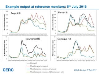
- #28: These graphs show variation in observed and modelled concentration through the day on one day only: 5th July 2016. The graphs show that for some sensors, e.g. Regent Street and Montague Rd, if the ref sensors are included in the inversion then the modelled conc can be made to fit the observed conc. At these sources the modelled conc is dominated by only one source. For the receptors where the inversion has a harder job making the modelled conc fit the observed conc (e.g. Newmarket Rd) it is because many sources impact on the receptor.


